An Overview of a Projected Balance Sheet
Definition
Projected Balance Sheet, also known as Proforma balance sheets, is a record that tracks the change of liability, assets, or equity of an organization or company over a certain period of time.
Components of Projected Balance Sheet
- Assets: Assets can be Fixed Assets like land or current property like software. They can also be categorized as tangible and nontangible.
- Liabilities: Liabilities can be explained as the things that the company owes. They could be mortgages, external debt, accrued taxes, etc.
- Equity: Equity represents the money that would return to the shareholders if all of the Assets (current & Fixed) are liquidated and all debts are paid.
How to Make a Projected Balance Sheet in Excel: Step-by-Step Procedure
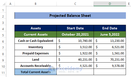
Step 1 – Prepare the Current Assets Dataset
- We have Cash, Inventory, Prepaid, Land, and Account Receivable values in the range of cells B6:B10.
- We’ve inserted values for these assets.
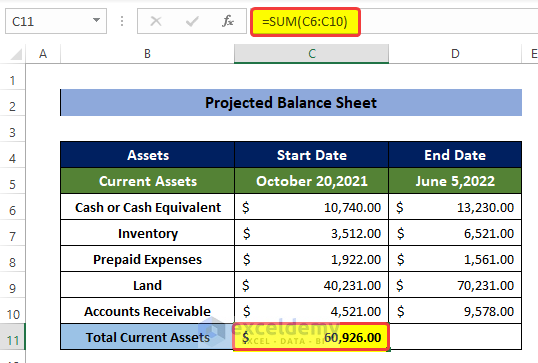
- Select the cell C11 and enter the following formula:
=SUM(C6:C10)
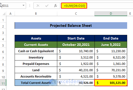
- Select the cell D11 and enter the following formula:
=SUM(D6:D10)
Read More: How to Make Stock Balance Sheet in Excel
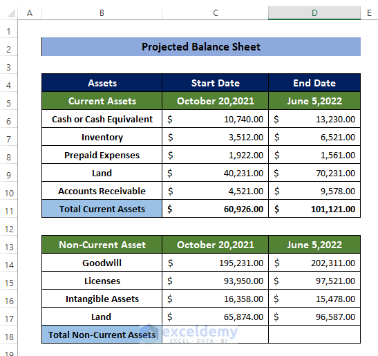
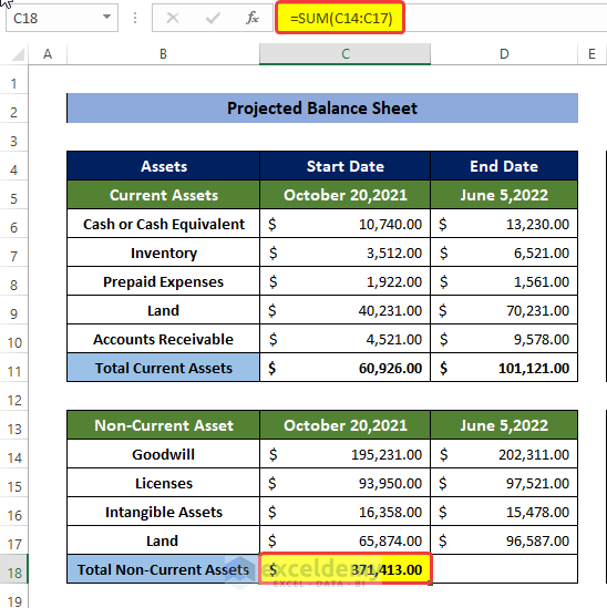
Step 2 – Estimate the Total Non-Current Assets
- List the non-current assets of the organization in a list format in the range of cells B14:B17.
- We put the values of non-current assets for October 20, 2021 in the range of cells C14:C17.
- The values of non-current Assets for June 5, 2022 are put in the range of cells D14:D17.
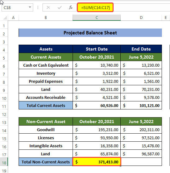
- Select the cell C18 and enter the following formula:
=SUM(C14:C17)
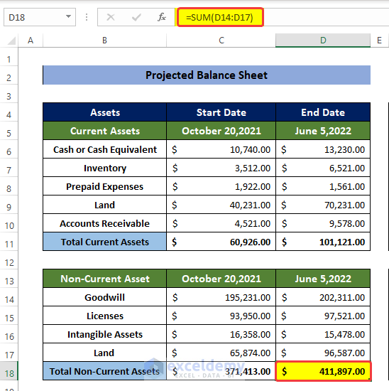
- Select the cell D18 and enter the following formula:
=SUM(D14:D17)
- Select the cell C20 and enter the following formula:
=SUM(C11,C18)
- Select the cell D20 and enter the following formula:
=SUM(D11,D18)
- This will calculate the sum of two types of Assets, Current and Non-Current Assets.
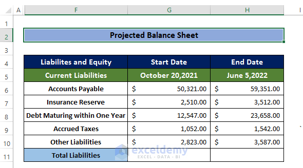
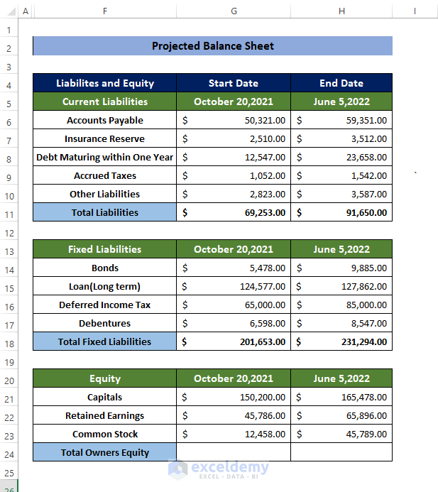
Step 3 – Evaluate Liabilities
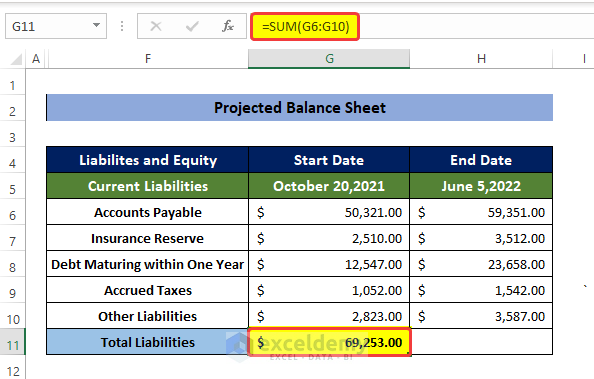
- List the Current Liabilities of the organization in a list format in the range of cells F6:F10.
- Put the values of those Current Liabilities on given dates in two ranges, G6:G10 and H6:H10.
- Select the cell G11 and enter the following formula:
=SUM(G6:G10)
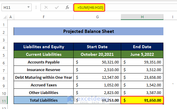
- Select the cell H11 and enter the following formula:
=SUM(H6:H10)
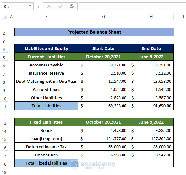
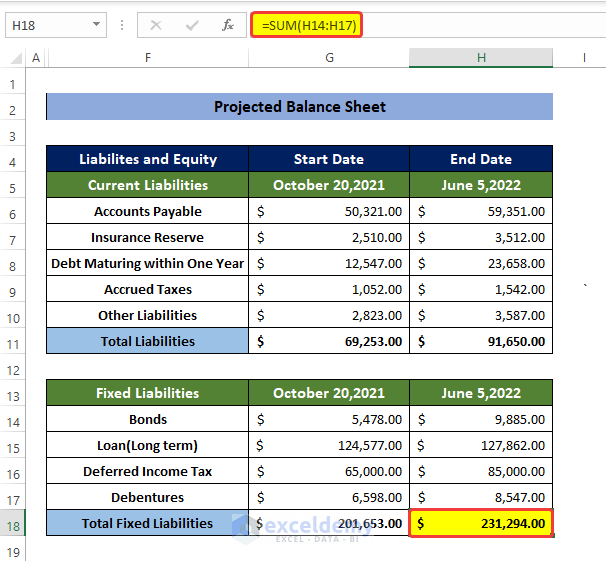
- List the Fixed Liabilities of the organization in a list format in the range of cells F14:F17.
- Use the ranges G14:G17 and H14:H17 for the values.
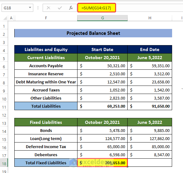
- Select the cell G18 and enter the following formula:
=SUM(G14:G17)
- Select the cell H18 and enter the following formula:
=SUM(H14:H17)
Read More: How to Tally a Balance Sheet in Excel
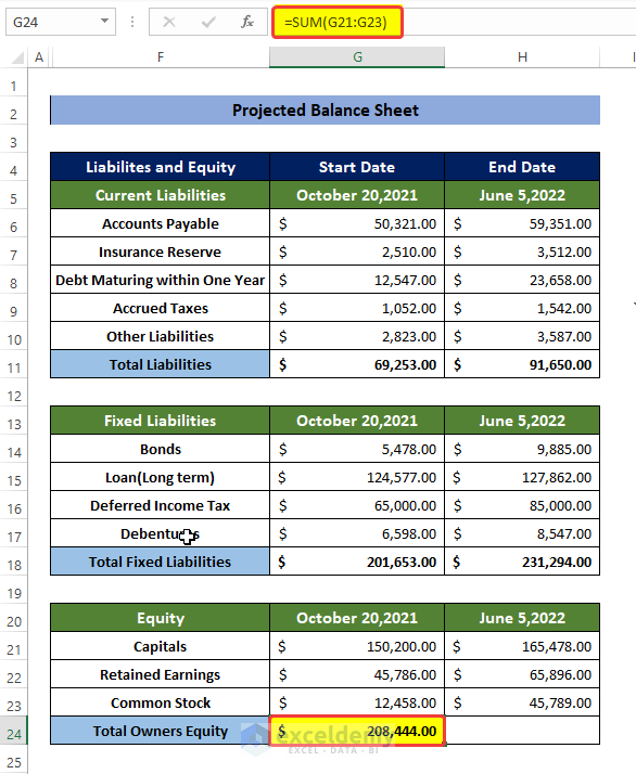
Step 4 – the Calculate Total Equity
- List the Equity of the organization in a list format in the range of cells F21:F23.
- Put the values in the ranges G21:G23 and H21:H23.
- Select the cell G24 and enter the following formula:
=SUM(G21:G23)
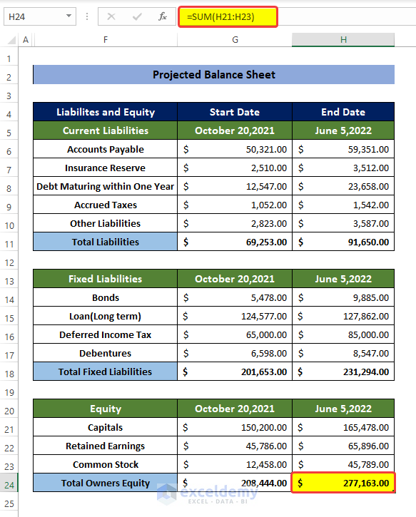
- Select the cell H24 and enter the following formula:
=SUM(H21:H23)
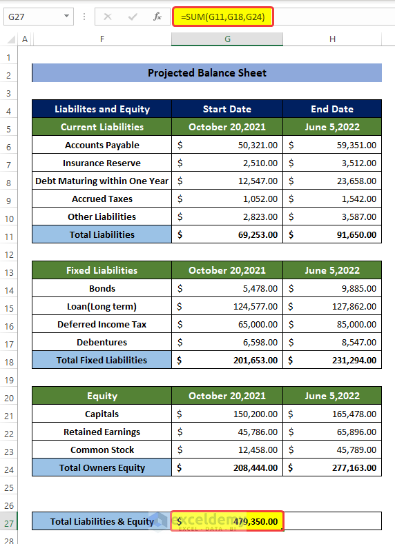
Step 5 – Calculate the Total Liabilities and Equity
- Select cell G27 and enter the following formula:
=SUM(G11,G18,G24)
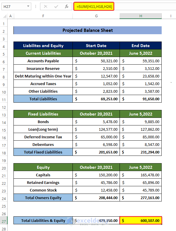
- Select cell H27 and enter the following formula:
=SUM(H11,H18,H24)
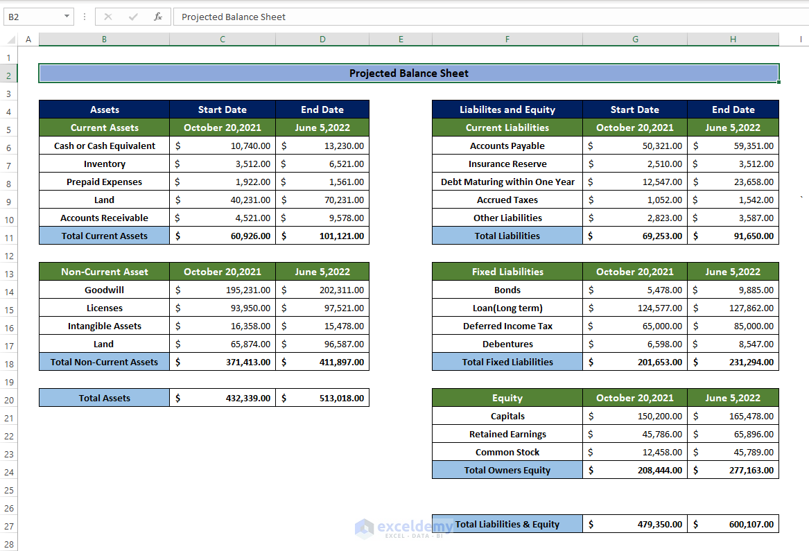
- Here’s the overview of the balance sheet.
Read More: Debit Credit Balance Sheet with Excel Formula
Download the Practice Workbook
Related Articles
- How to Prepare Balance Sheet from Trial Balance in Excel
- How to Calculate Running Balance Using Excel Formula
- How to Keep a Running Balance in Excel
- Calculate Debit Credit Running Balance Using Excel Formula
- How to Make Profit and Loss Account and Balance Sheet in Excel
- How to Make Trial Balance in Excel
<< Go Back To How to Make Balance Sheet in Excel |Excel For Finance | Learn Excel
Get FREE Advanced Excel Exercises with Solutions!
