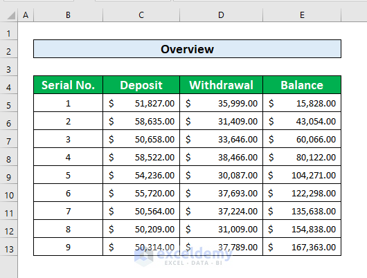
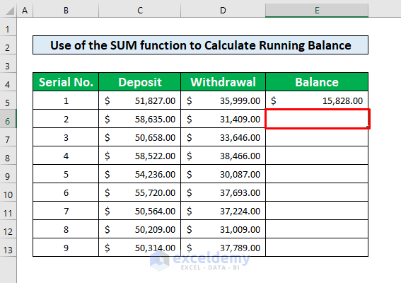
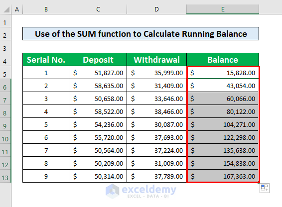
Consider the following dataset of cash flow inside some bank accounts. The deposits and withdrawals are listed in columns C and D. We’ll calculate their running balance.
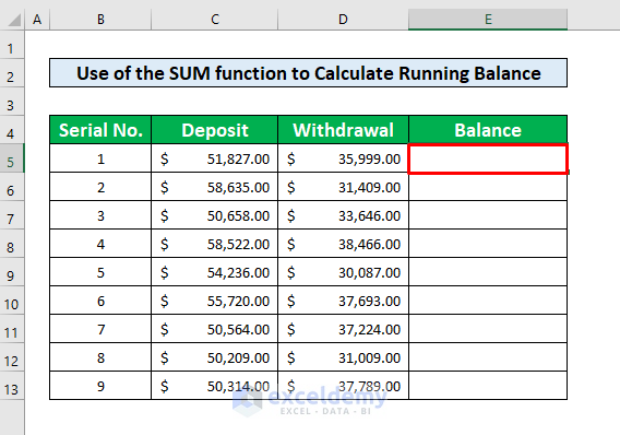
Method 1 – Using the SUM Function to Calculate a Running Balance in Excel
Steps:
- Select cell E5.
- Use the following formula in the cell.
=SUM(C5-D5)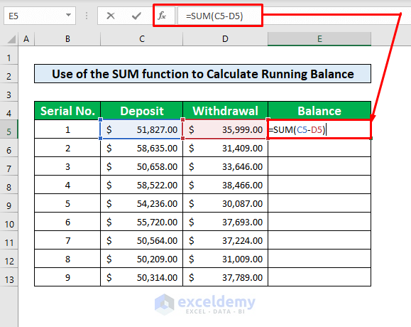
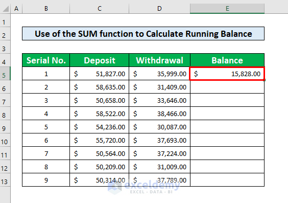
- Press Enter on your keyboard and you’ll get $15,828.00 as the return of the SUM function in cell E5.
- Select cell E6.
- In the Formula Bar, use the following formula:
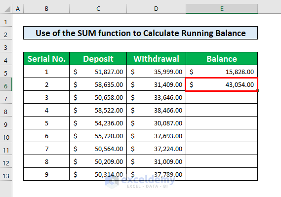
=SUM(C6-D6+E5)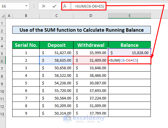
- Press Enter.
- Place your cursor on the bottom-right corner of cell E6, and the Fill Handle icon will appear.
- Drag the icon down.
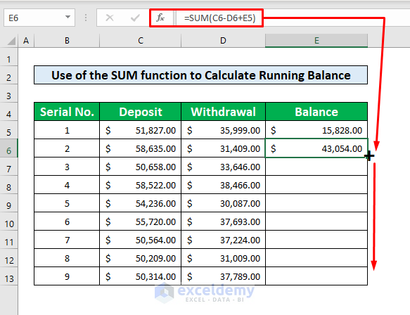
- Here’s the final result.
Read More: How to Keep a Running Balance in Excel
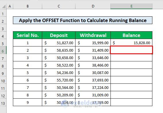
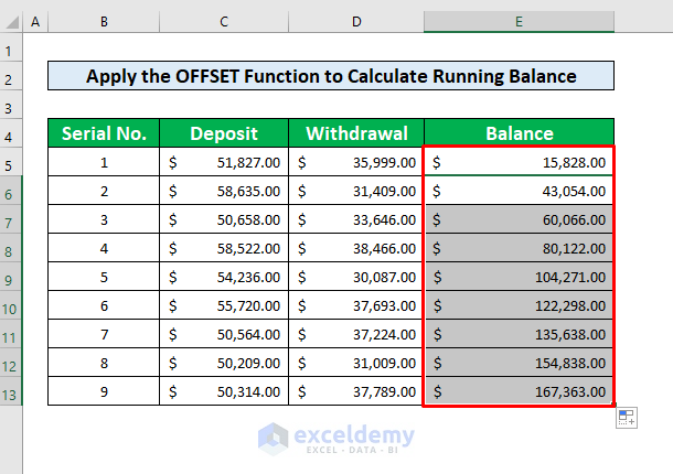
Method 2 – Apply the OFFSET Function to Calculate a Running Balance in Excel
Steps:
- Use the sum formula above for cell E5.
- Select cell E6.
- Use the following formula inside the cell:
=SUM(C6,-D6,OFFSET(E6,-1,0))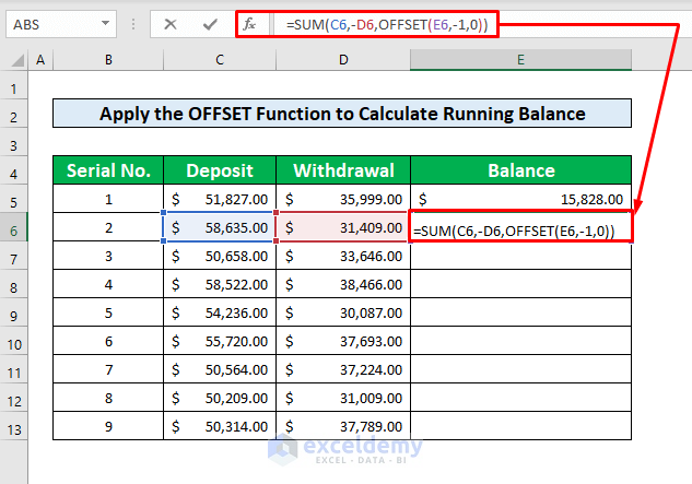
- Press Enter. You will get $43,054.00 as the output of the function in cell E6.
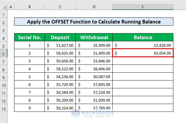
- Use the Fill Handle to AutoFill the rest of the cells from E6 to E13.
Read More: Calculate Debit Credit Running Balance Using Excel Formula
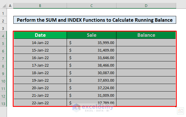
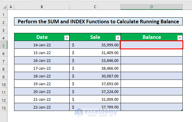
Method 3 – Use the SUM and INDEX Functions to Calculate a Running Balance in Excel
We’ll use a single bank account and a sequential list of deposits to calculate the account’s running total.
Steps:
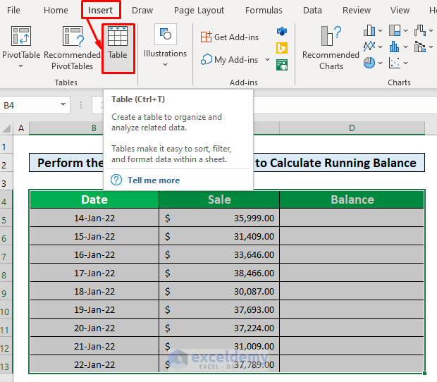
- Select the cell array B4 to D13.
- From the Insert tab go to Table.
- A window pops up titled Create Table.
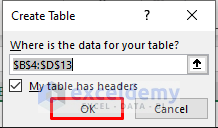
- Press the OK button
- Select cell D5.
- Insert the following function into the cell:
=SUM(INDEX([Sale],1):[@Sale])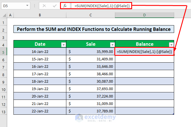
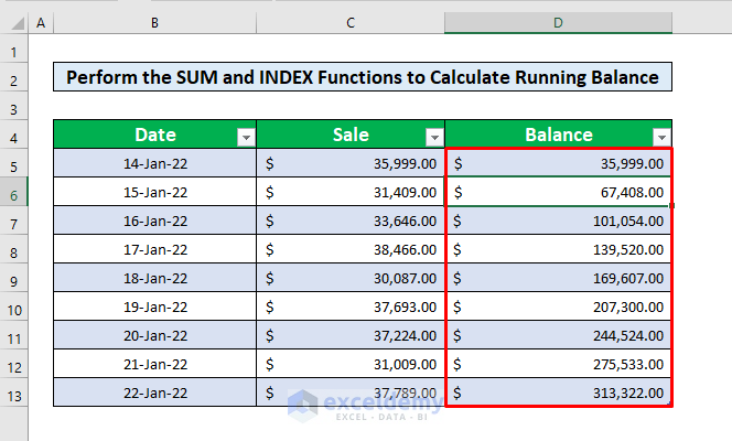
- Press Enter on your keyboard, and you will be able to calculate the running balance to the entire column which has been given below screenshot.
Read More: Debit Credit Balance Sheet with Excel Formula
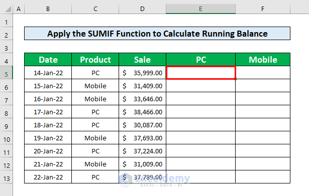
Method 4 – Apply the SUMIF Function to Calculate Running Balance in Excel
We have a data collection for which we want to calculate the running balance for PC and Mobile in two separate columns, E and F.
Steps:
- Select cell E5.
- Insert the following formula into the cell:
=SUMIF($C$5:C5, $E$4, $D$5:D5)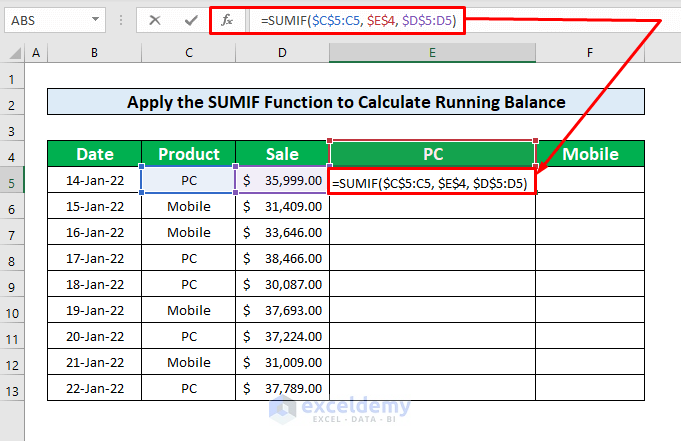
- Press Enter on your keyboard to get the first result.
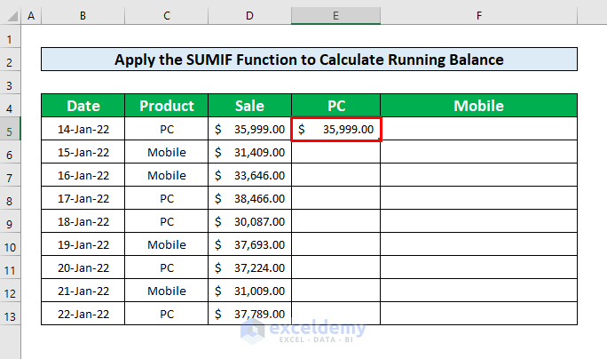
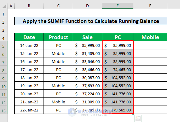
- AutoFill to the rest of the column.
- Select cell F5.
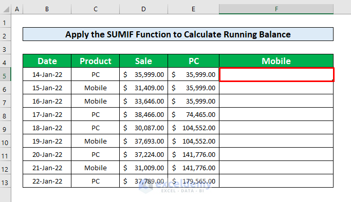
- Insert the following formula into that cell:
=SUMIF($C$5:C5, $F$4, $D$5:D5)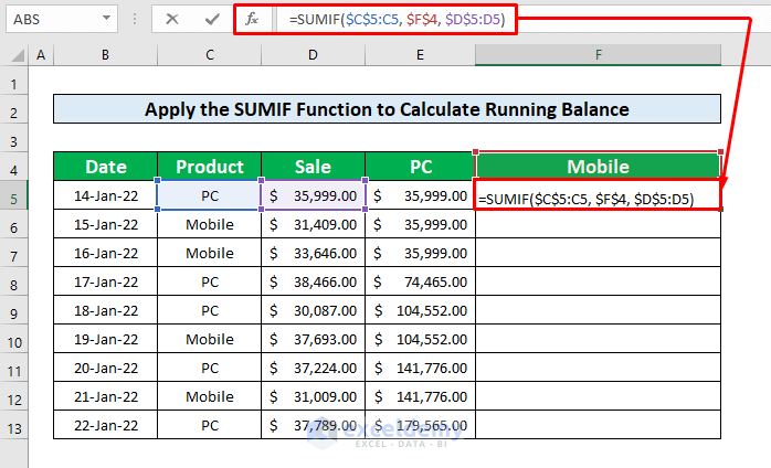
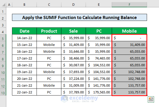
- Press Enter.
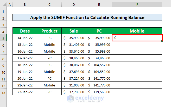
- AutoFill the column to get the results.
Download the Practice Workbook
Download this practice workbook follow along while reading the article.
Related Articles
- How to Prepare Balance Sheet from Trial Balance in Excel
- How to Make Stock Balance Sheet in Excel
- How to Make Projected Balance Sheet in Excel
- How to Make Profit and Loss Account and Balance Sheet in Excel
- How to Tally a Balance Sheet in Excel
- How to Make Trial Balance in Excel
<< Go Back To How to Make Balance Sheet in Excel |Excel For Finance | Learn Excel
Get FREE Advanced Excel Exercises with Solutions!
