How to Create Format for Projected Financial Statements in Excel

Part 1 – Creating a Projected Income Statement Format

Steps:

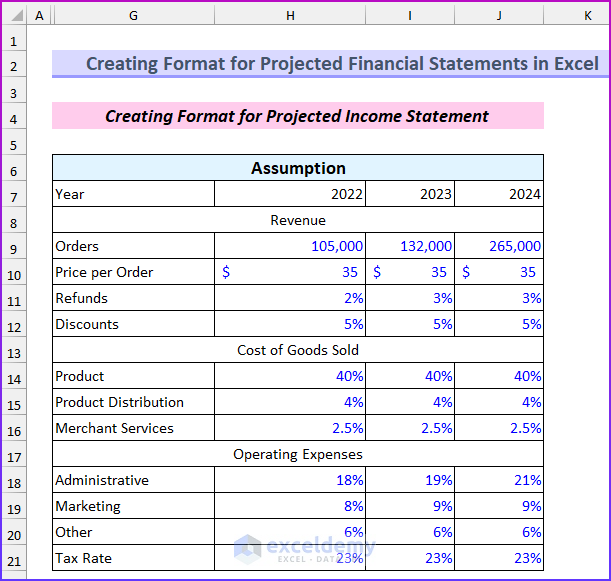
• Insert all the assumptions. These values will be referenced in the income statement.

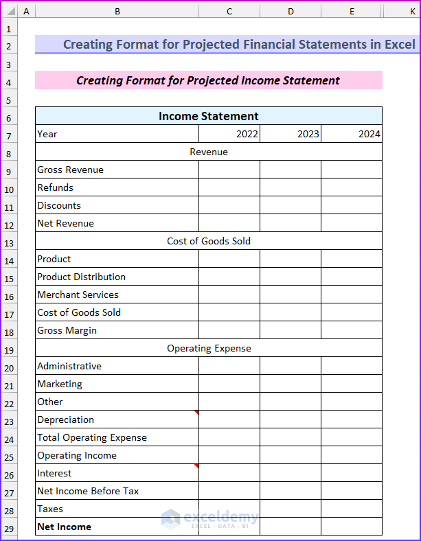
• Input all the fields for the income statement. We will forecast for the years 2022, 2023, and 2024.

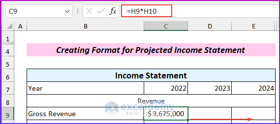
• Insert this formula in cell C9 to calculate the gross revenue and drag the Fill Handle to the right to AutoFill the formula.

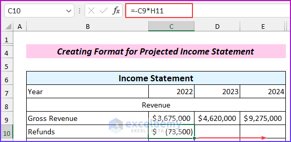
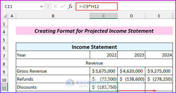
• Use another formula in cell C10 to calculate the refunds.

• Use the following formula in cell C11 to find discounts.

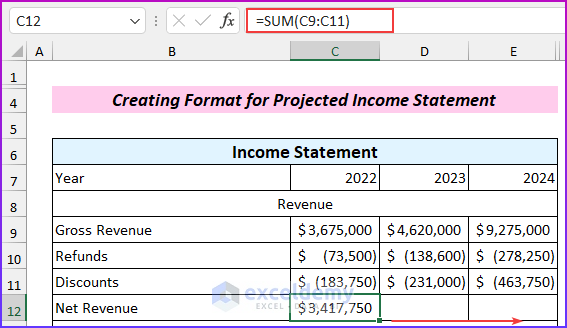
• Insert this formula in cell C12 to find the net revenue.

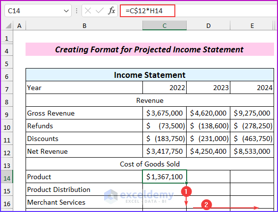
• Insert this formula in cell C14.

• Drag the formula two rows down and fill to the right.

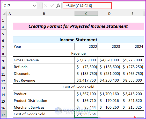
• Use the following formula to calculate the cost of goods sold.

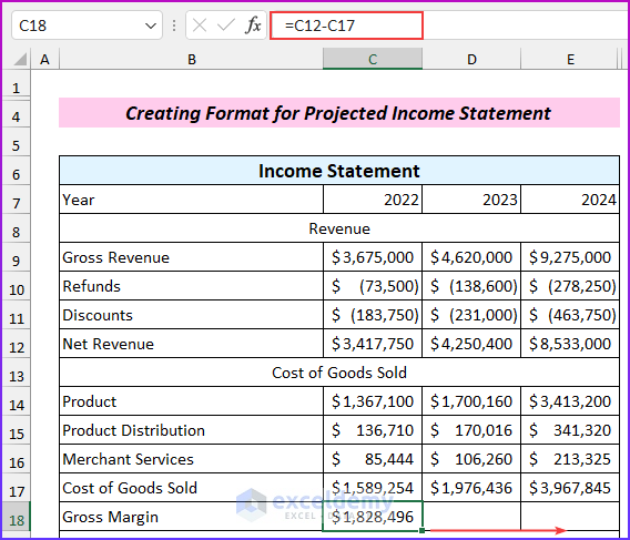
• Use this formula to find the gross margin.

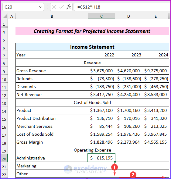
• Insert the following formula in cell C20, then drag it two rows down and to the right.

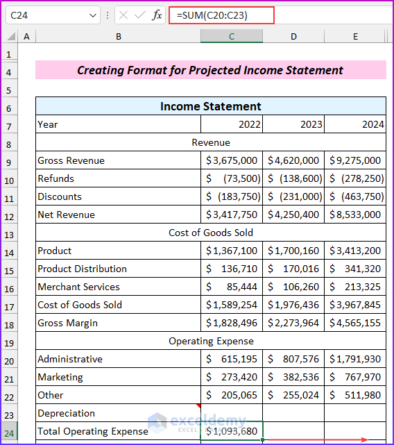
• Use the following formula to calculate the total operating expense.

• We will find the values for the depreciation and interest expense later, so keep those blank for now.

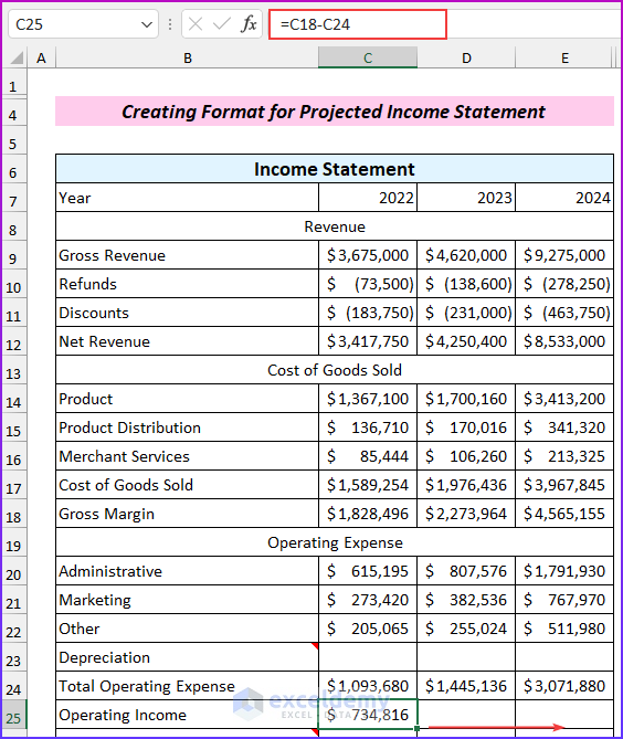
• Use this formula in cell C25 to find the operating income.

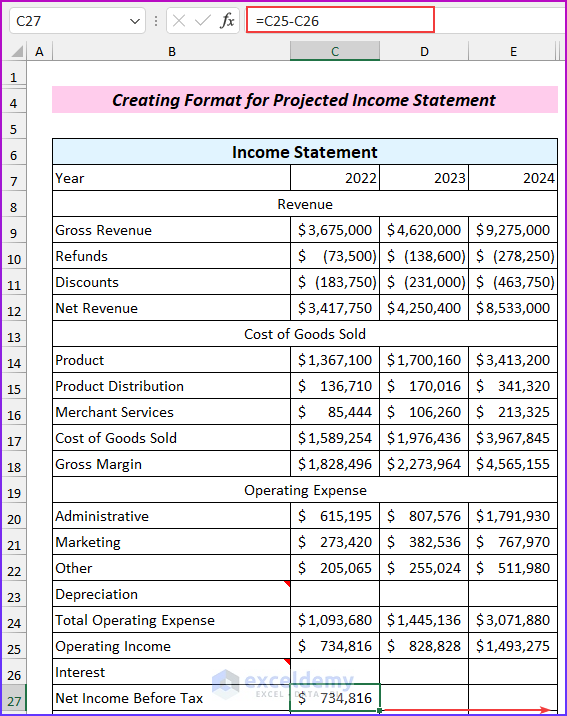
• Insert this formula to find the net income before tax.

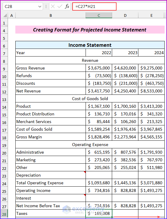
• Use this formula in cell C28 to find the tax amount.

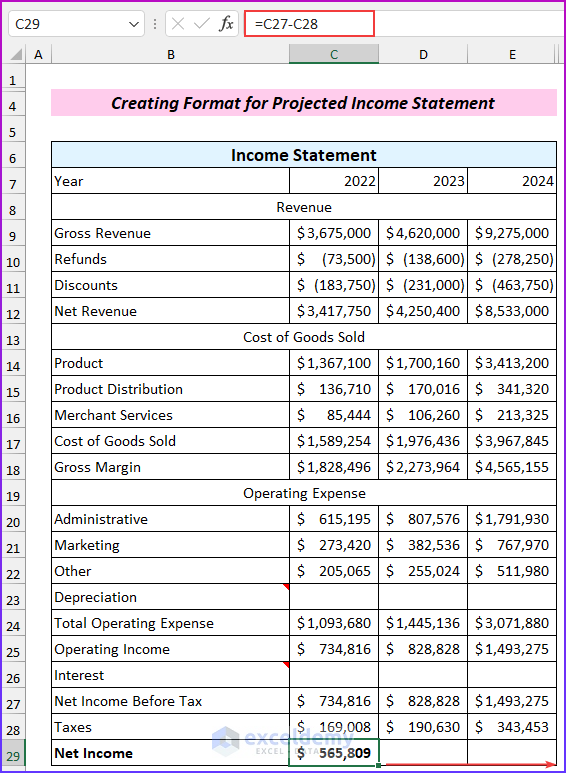
• Use this formula in cell C29 to find the net income without considering depreciation and interest.

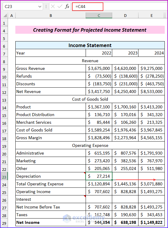
• We will find the values of the depreciation from this part. Link to those values by using this formula.

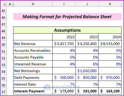
• Use the information from this part for the interest amount, so insert the following formula:

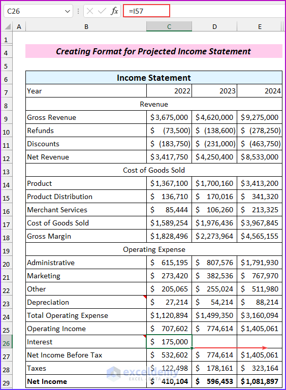
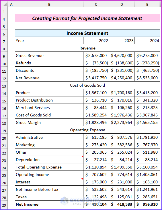
• Here’s the finalized statement.

Part 2 – Making a Format for the Projected Balance Sheet

We need historical data from last year, which is 2021 for this article. We will need the “net cash flow” from the cash flow statement to calculate the “cash & cash equivalents” on the balance sheet. We will also need to refer to the income statement for other values.

Steps:

• We have projected the capital expenditure and depreciation. The blue text indicates assumed values. We have the total depreciation values from this in our income statement.

• List all the assumptions for the balance sheet. From these assumptions, we have found the interest expenses for the income statement.

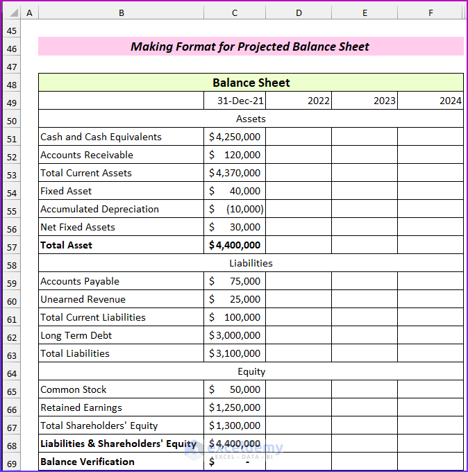
• Insert all the fields for the balance sheet. We have used last year’s (2021) values. There is a field called “balance verification” that we will use to check whether the balance sheet evens out.

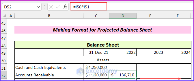
• Use this formula in cell D52 and drag it to the right.

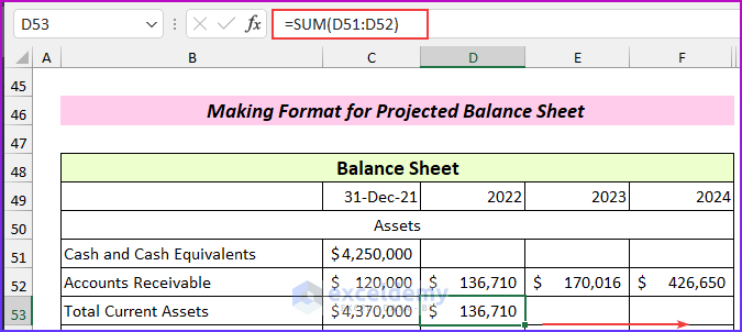
• Use this formula to find the total current assets.

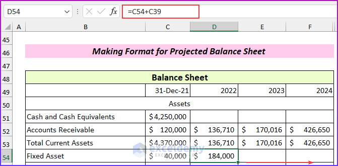
• Use another formula to find the fixed assets.

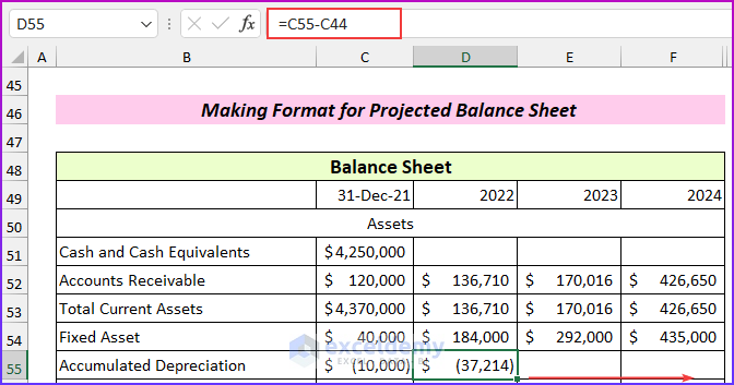
• Use this formula to find the accumulated depreciation.

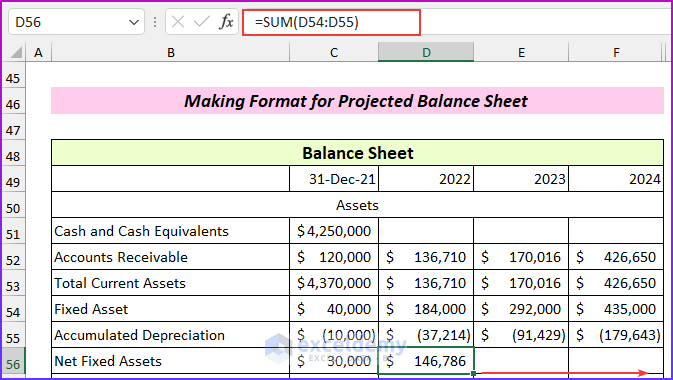
• Insert this formula in cell D56 to get the values of net fixed assets.

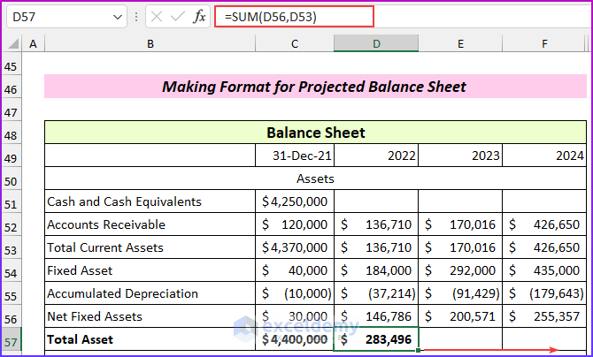
• Insert this formula to calculate the total assets.

• Similarly, we will use formulas to calculate the values for the liabilities and equity parts. The balance verification is not zero yet (0 means the balance sheet balances). This is because we have kept the cash and cash equivalents empty.

• From the cash flow statement, extract the net cash flow values. Input those values with the following formula in cell D51 and fill to the right.

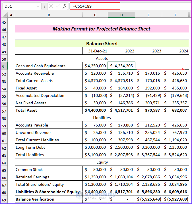
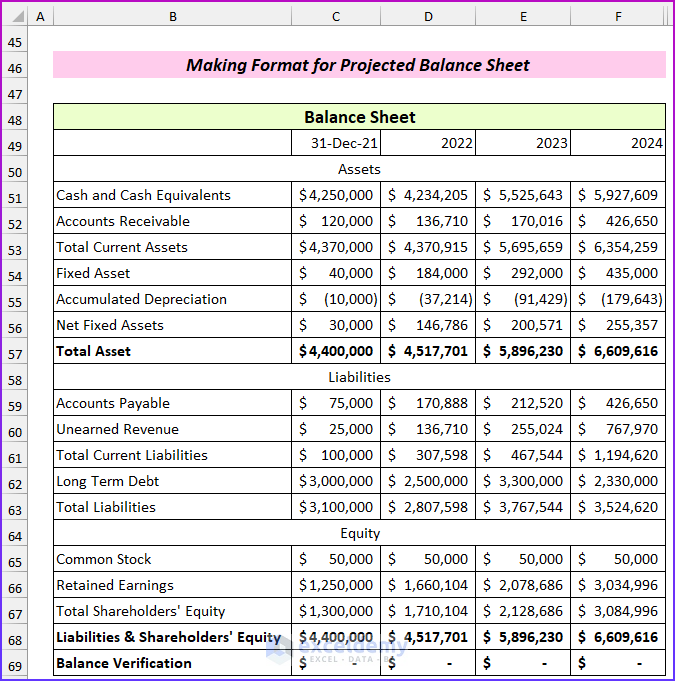
• Here’s the finalized sheet.

Part 3 – Preparing the Projected Cash Flow Statement

We will take most of the items from the balance sheet. Net income will come from the income statement, and depreciation will come from the “capital expenditure and depreciation” that we created in the second part.

Steps:

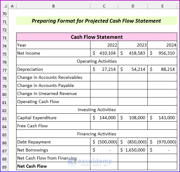
• Insert all the fields for the cash flow statement.
• Link the known values:
  • Net Income → Income Statement
  • Depreciation → Projected Capex and Depreciation
  • Capital Expenditure → Projected Capex and Depreciation
  • Debt Repayment → Balance Sheet Assumption (negative value)
  • Net Borrowings → Balance Sheet Assumption

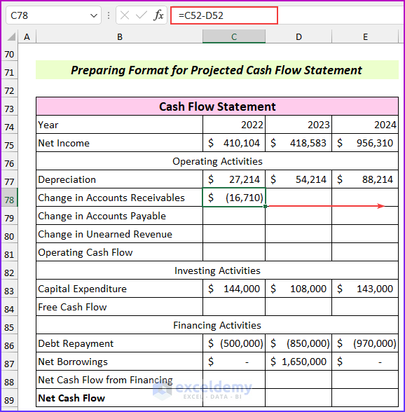
• Use this formula in cell C78 to find the change in accounts receivable and drag it to the right to AutoFill.

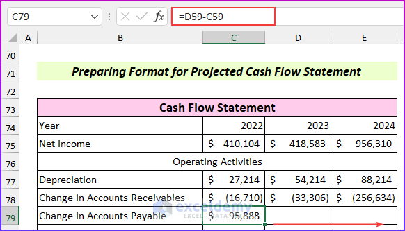
• Use this formula to calculate the change in accounts payable.

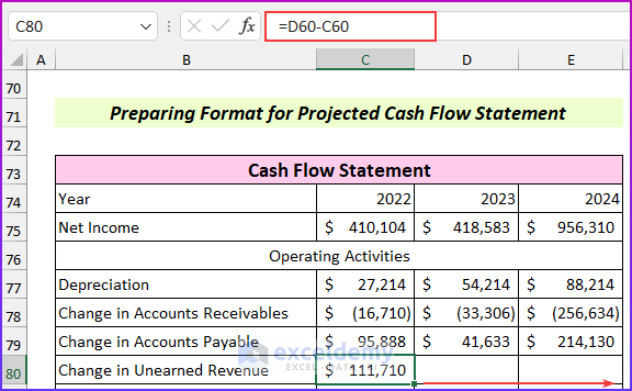
• Insert this formula to find the change in unearned revenue.

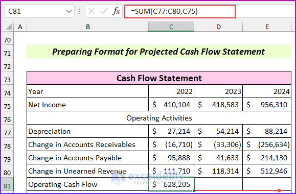
• Use this formula in cell C81 to find the operating cash flow.

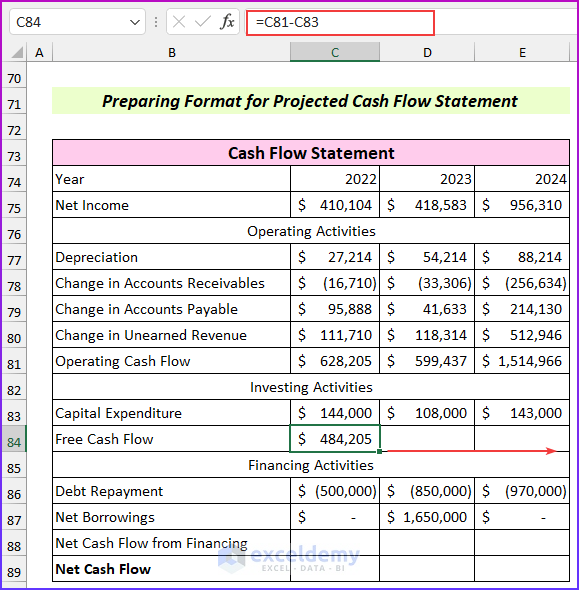
• Insert this formula to find the free cash flow.

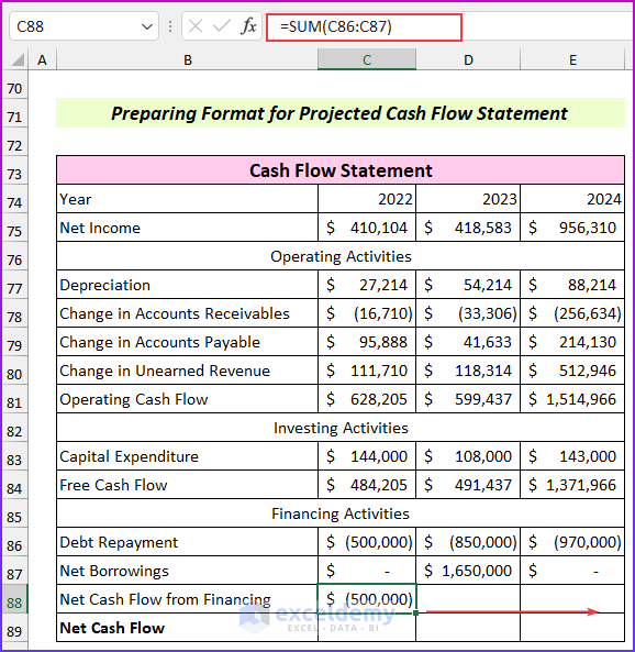
• Use the following formula to calculate the net cash flow from financing.

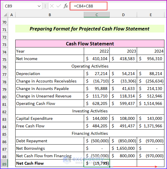
• Use this formula in cell C89 to find the net cash flow.

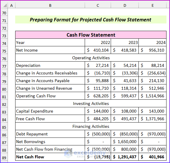
• Here’s the final resulting after using AutoFill to fill in the columns to the right.

Projected Financial Statements for Five Years

We have projected the financial statements for three years in this article. You can easily extend this for two more years to make it a five-year projection. You can insert new columns and drag the formulas to the right. This will create the five-year forecasting for the financial statements. The model’s accuracy will decline, so keep that in mind.

Download the Practice Workbook

Related Articles

• Construction Company Financial Statements in Excel

<< Go Back to Financial Statement | Finance Template | Excel Templates