Step 1 – Enter Values for Current and Non-current Assets
A balance sheet has three parts: records of assets, liabilities, and stakeholders’ equity.
- We are taking two data points for two years.
- The sheets can also be prepared for one entry. Either way, you can add all the assets in a separate category or in one, depending on how you want to present it.
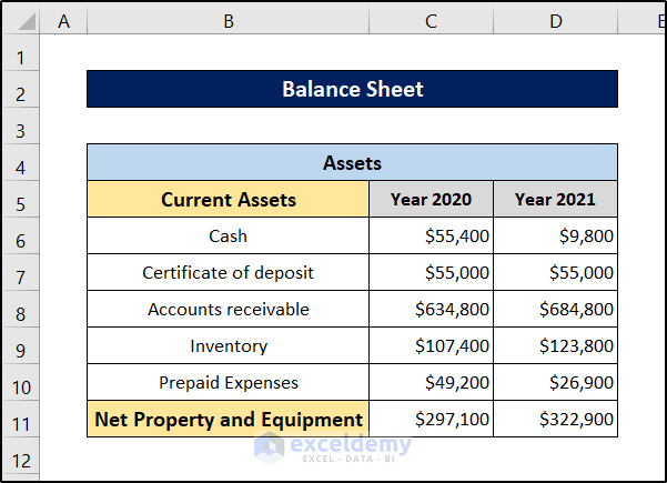
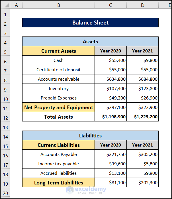
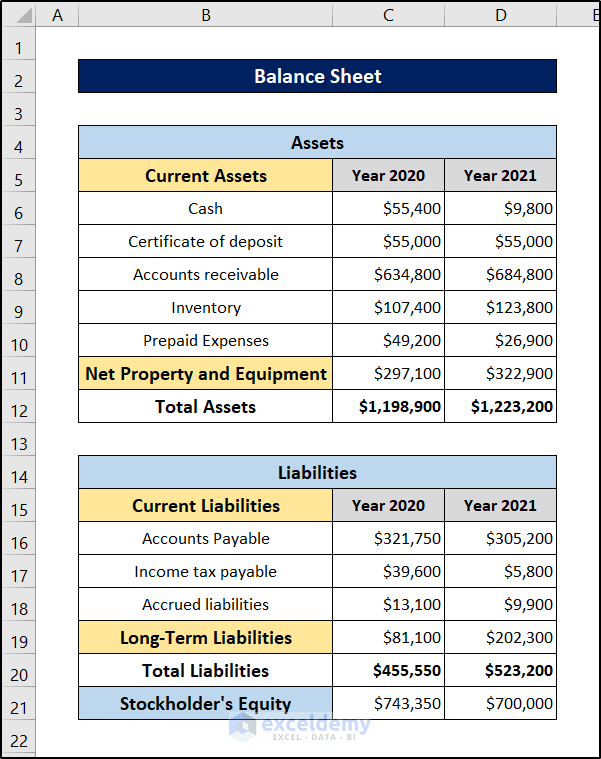
- We have added cash, certificate of deposit, accounts receivable, inventory, and prepaid expenses as the current assets.
- We also added net property and equipment as the non-current asset.
- Our asset chart of the balance sheet will look like this.
Step 2 – Calculate Total Assets
- Select cell C12 and insert the following formula.
=SUM(C6:C11)
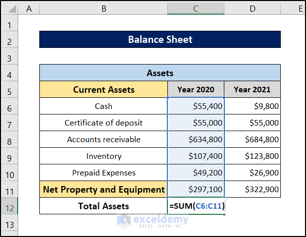
- Press Enter and you will get the total assets for the year 2020.
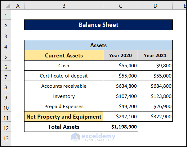
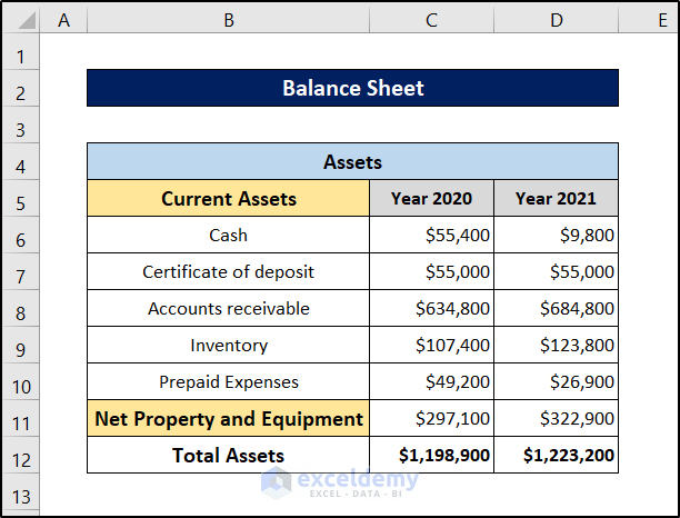
- Select the cell again and click and drag the fill handle icon to the cell on the right. You will get the value for the year 2021.
Step 3 – Document Current and Long-Term Liabilities
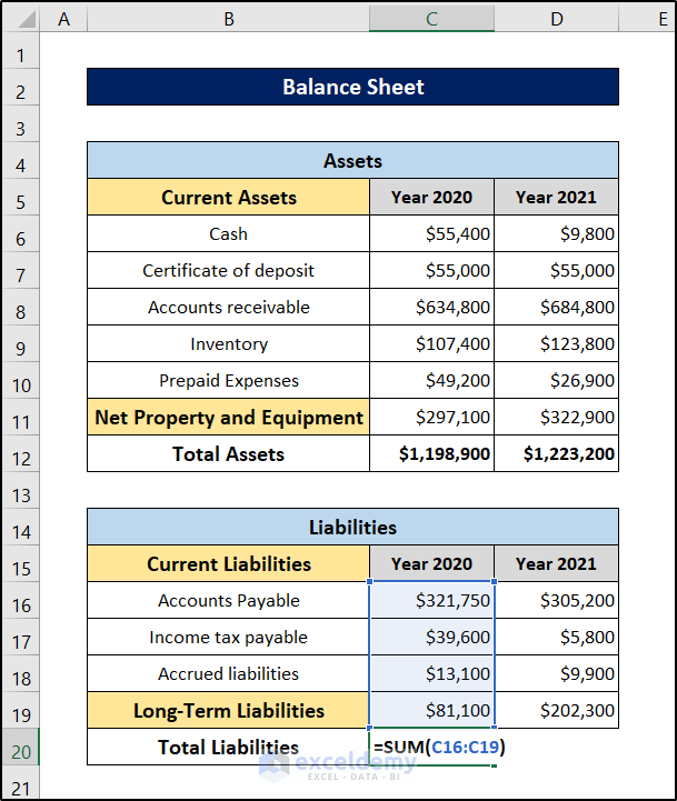
- We’ve entered the values of the liabilities, and the balance sheet will now look like this.
- We have included accounts payable, income tax payable, and accrued liabilities as the current liabilities and only one section for long-term liabilities.
Step 4 – Estimate Total Liabilities
- Select cell C20 and insert the following formula.
=SUM(C16:C19)
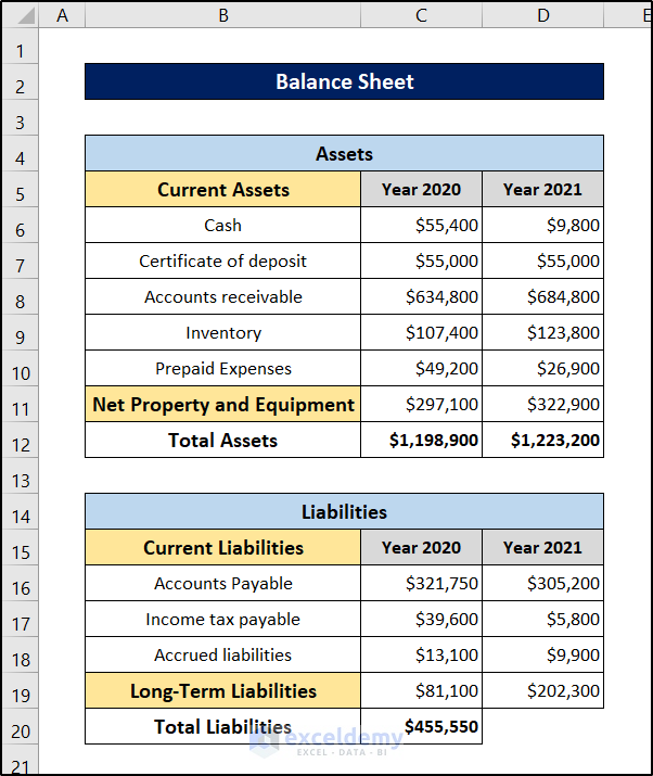
- Press Enter and you will get the total liabilities for the year.
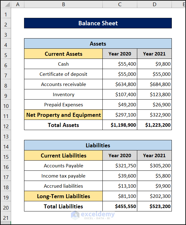
- Select the cell again and click and drag the fill handle icon to the right to replicate the formula for the next year.
Step 5 – Record the Stakeholder’s Equity
Another portion of the balance sheet is the stakeholder’s equity. Generally, a balance sheet is balanced by the liabilities and stakeholders’ equity sum and assets. This portion can also include various sub-portions, but we have included only one section for demonstration.
You can document all the different parts if you have many sub-parts and add them to find the final stockholder’s equity too.
Step 6 – Calculate Total Liabilities and Equity
- Select cell C22 and insert the following formula.
=SUM(C20:C21)
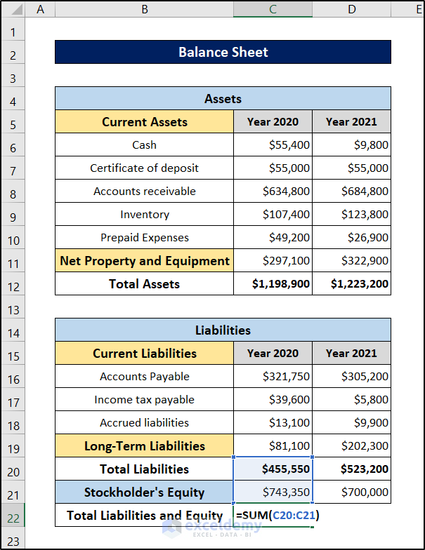
- Press Enter and you will get the result for the year 2020.
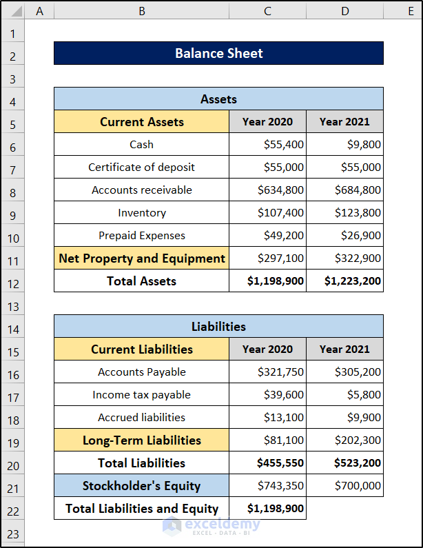
- Select the cell again.
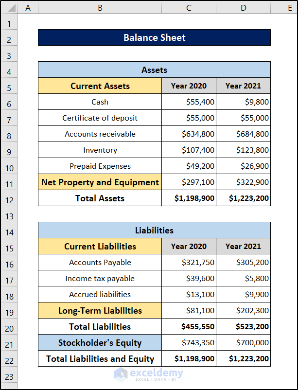
- Click and drag the fill handle icon to the right to replicate the formula for the year 2021.
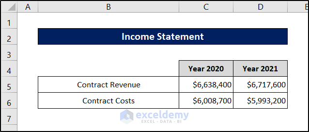
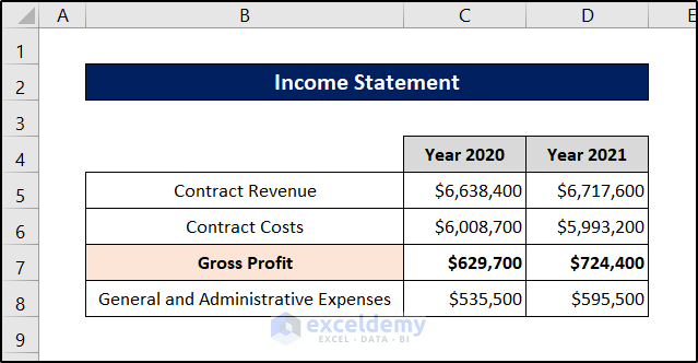
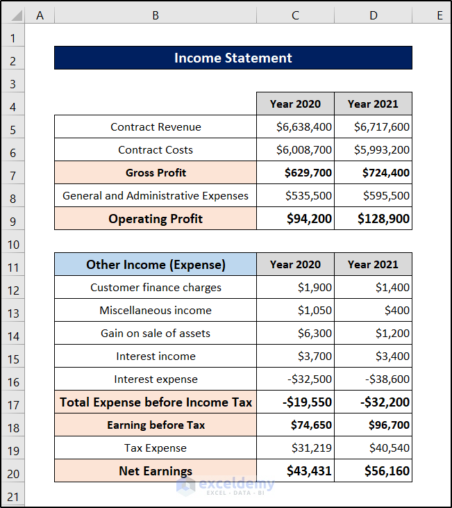
Step 7 – Record Gross Profits
The income statements have the records of income, expenses, and tax records.
- Let’s assume the company profits from contracts revenue directly. Document the contract revenues and costs in the income statement.
- Select cell C7 and use the following formula to subtract the costs from the revenue.
=C5-C6
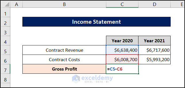
- Press Enter.
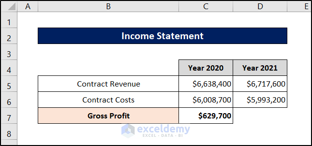
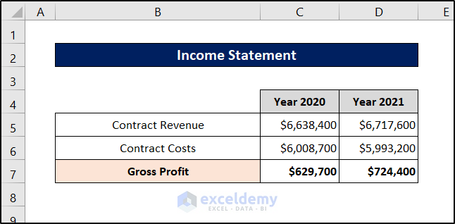
- Select the cell again and click and drag the fill handle icon to the right to replicate the formula for the year 2021.
Step 8 – Calculate the Operating Profit
- Add the expenses under the profit section.
- Select cell C9 and use the following formula.
=C7-C8
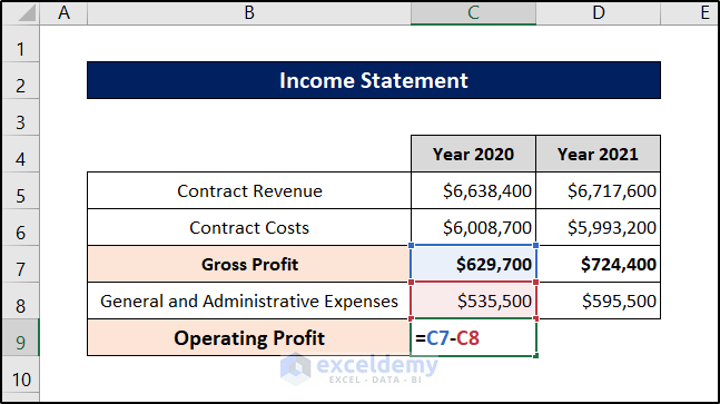
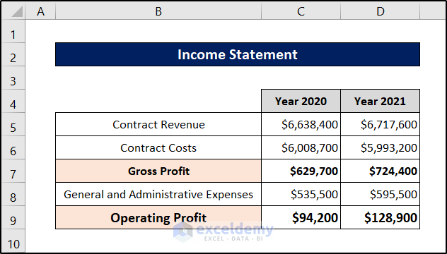
- Press Enter.

- Select the cell again and click and drag the fill handle icon to the right to replicate the formula for the next cell.
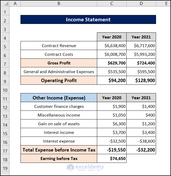
Step 9 – Determine Other Income/Expenses
- Add all the expenses below the previous section in the income statement.
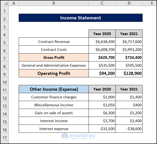
We have put in all the income values in positive numbers and the expense values in negative numbers. Putting these cells in negative and summing them up makes it easier later on.
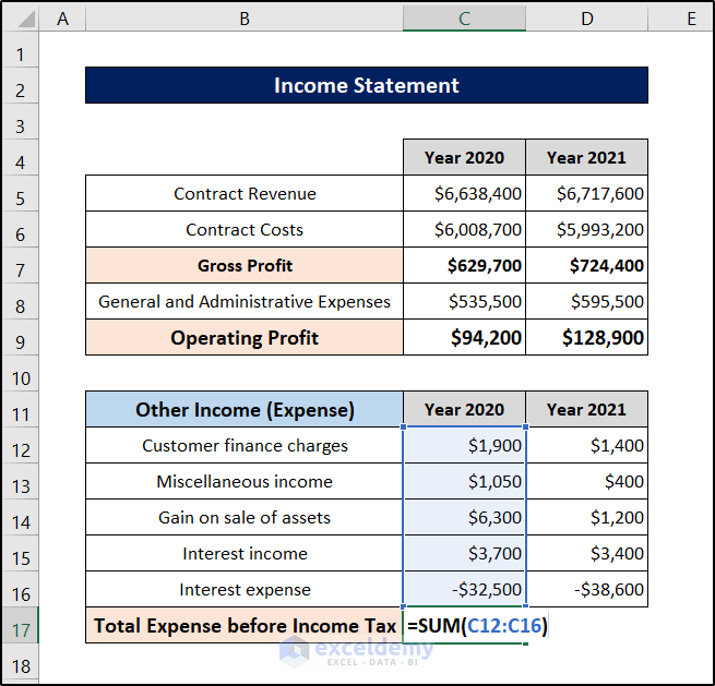
Step 10 – Evaluate Expense Before Tax
- Select cell C17 and use the following formula.
=SUM(C12:C16)
- Press Enter.
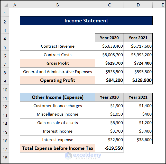
- Select the cell again.
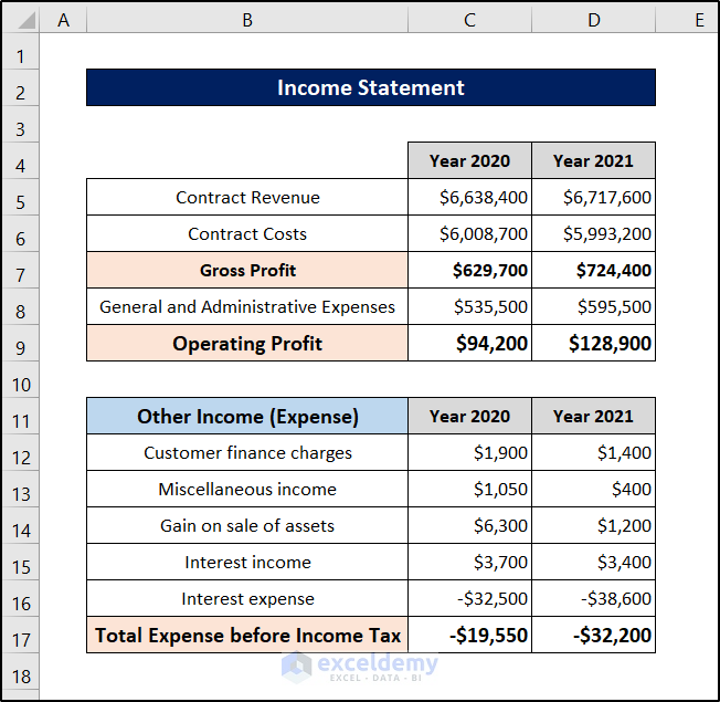
- Click and drag the fill handle icon to the right to replicate the formula for the next year.
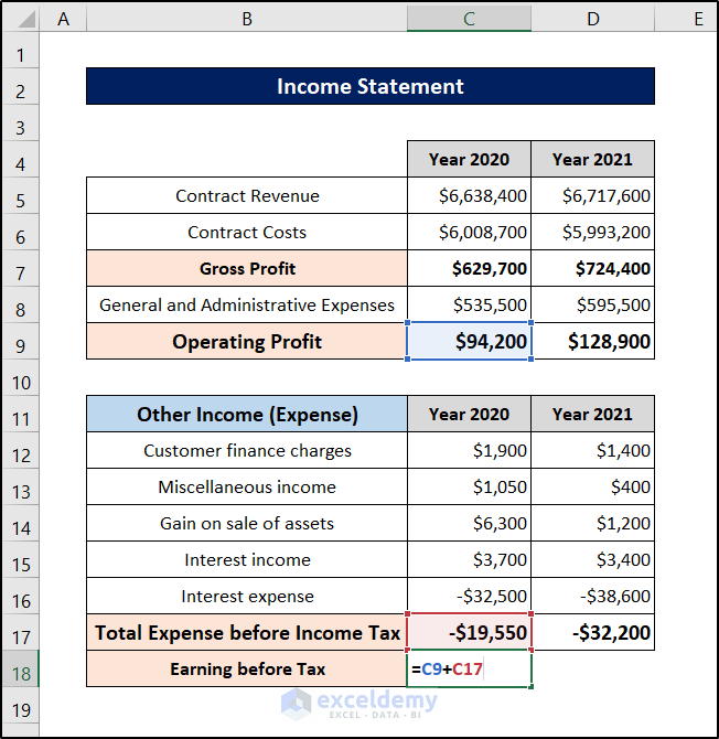
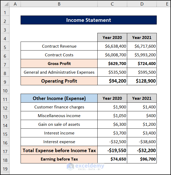
Step 11 – Calculate Earnings Before Tax
- Select cell C18 and use the following formula.
=C9+C17
- Press Enter.
- Select the cell again and click and drag the fill handle icon to the right to replicate the formula for the next year.
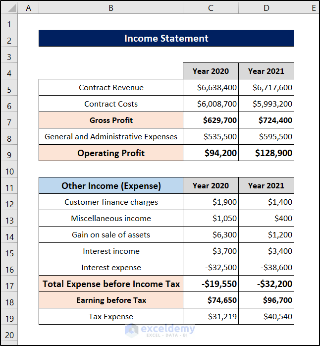
Step 12 – Determine Net Earnings
- Enter tax expense values in the income statement below the previous portion.
- Select cell C20 and use the following formula.
=C18-C19
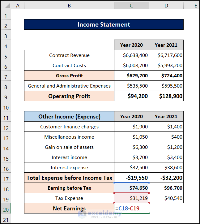
- Select the cell again and click and drag the fill handle icon to the right to find the net earnings for the next year.
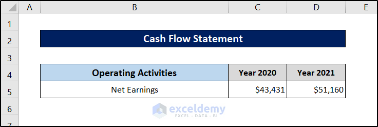
Step 13 – Record Net Earnings for the Cash Flow Statement
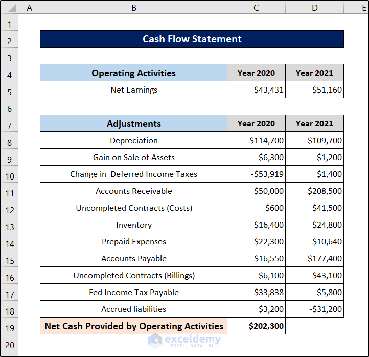
- Put the net earning values in the cash flow statement.
Step 14 – Enter the Adjusted Values
- Enter all the adjusted values for the cash flow segment.
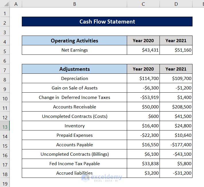
We have added a plethora of values in this section. There are some negative values for an easier summation later on.
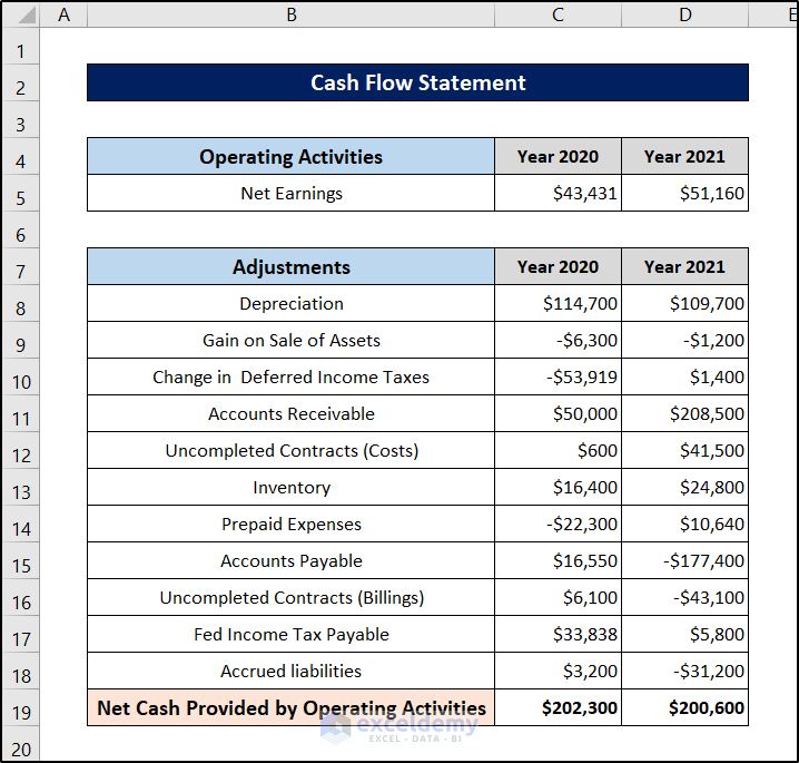
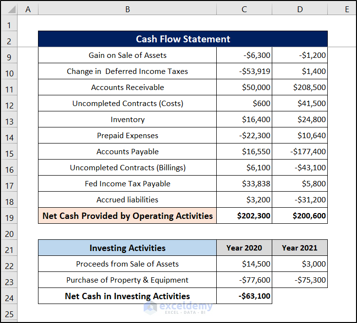
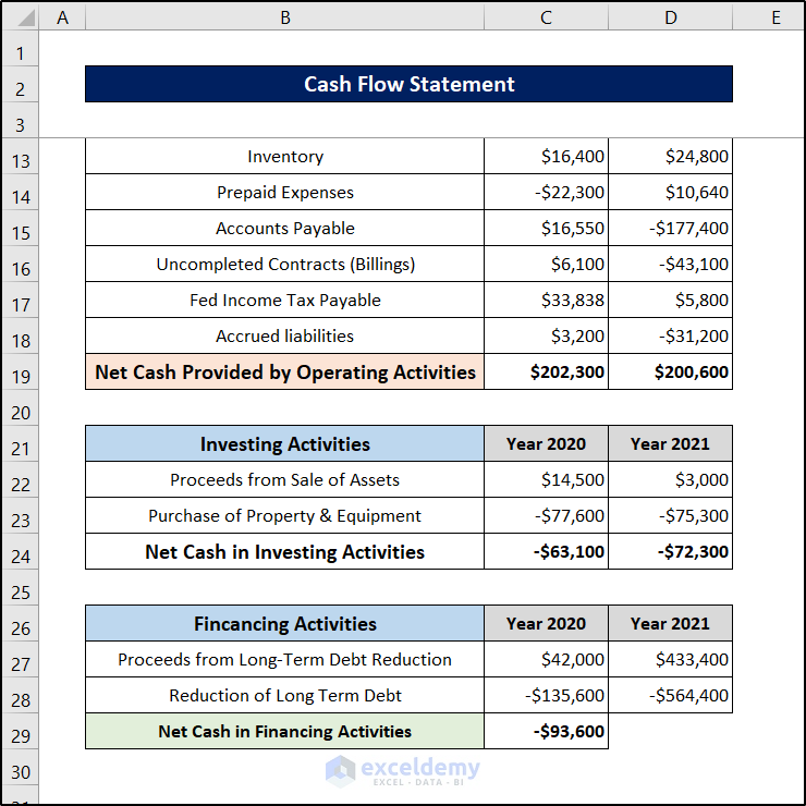
Step 15 – Compute the Net Cash Provided by Operating Activities
- Select cell C19 and insert the following formula.
=SUM(C5:C18)
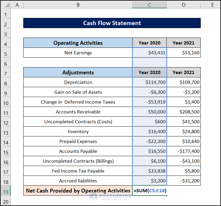
Press Enter.
- Select the cell again and click and drag it to the right to replicate the formula for the next cell.
Step 16 – Record Investing Activities
- Put investing activities under the cash flow statement.
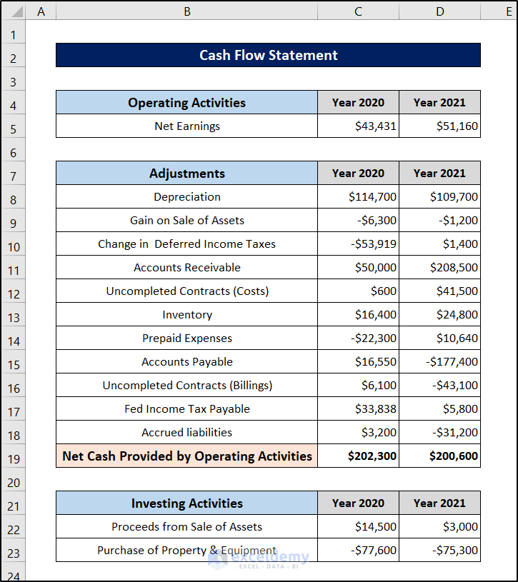
We have added the purchase cost as a negative value since it’s going to be subtracted from the sale values.
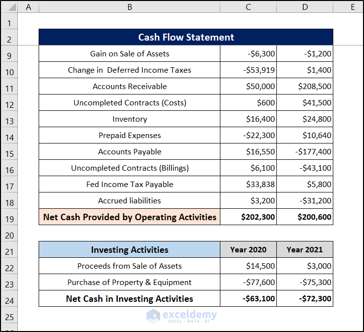
Step 17 – Calculate the Net Cash in Investing Activities
- Select cell C24 and use the following formula.
=SUM(C22:C23)
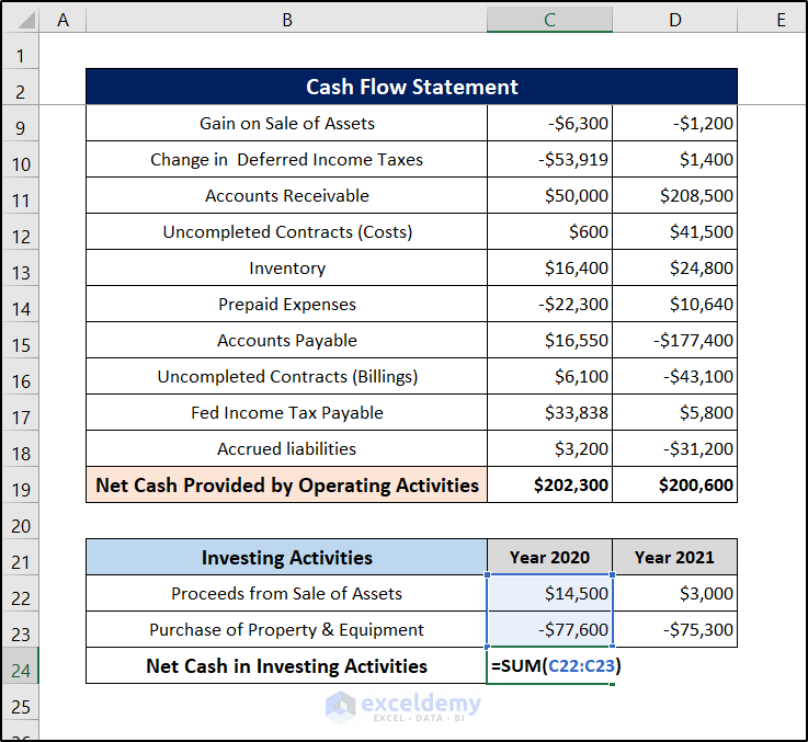
- Press Enter.
- Select the cell again and click and drag the fill handle icon to the right of it to replicate the formula for the next year.
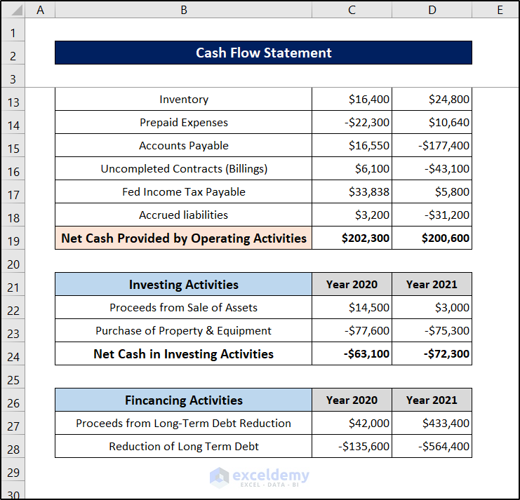
Step 18 – Record Financing Activities
- Put financing activities under the previously created section of the cash flow statement.
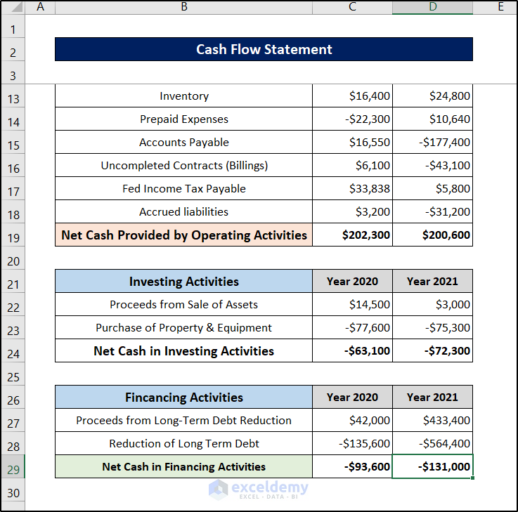
Step 19 – Determine the Net Cash in Financing Activities
- Select cell C29 and use the following formula.
=SUM(C27:C28)
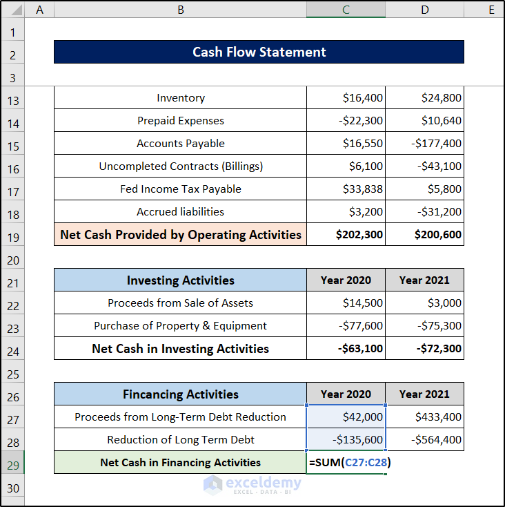
- Press Enter.
- Select the cell again and click and drag the fill handle icon to the right to replicate the formula for the next year.
Step 20 – Document the Net Increase in Cash
- Record the net increase in cash in the next section of the cash flow statement.
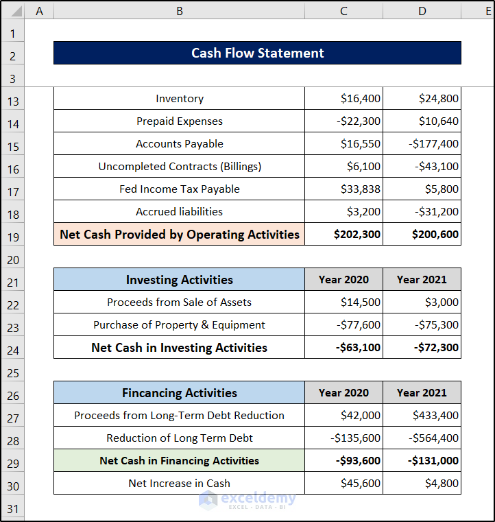
Step 21 – Record Cash at Beginning of the Year
- Record the cash amount at the beginning of each year in the final portion of the cash flow statement.
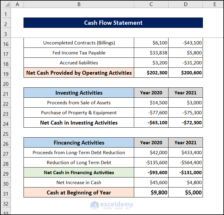
Step 22 – Evaluate Cash at End of the Year
- Select cell C32.
- Insert the following formula.
=SUM(C30:C31)
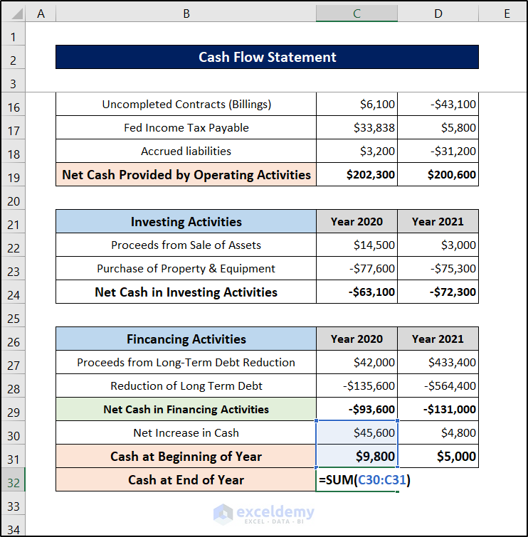
- Press Enter.
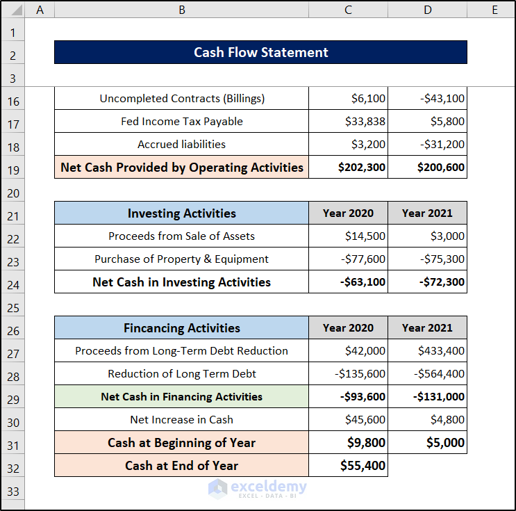
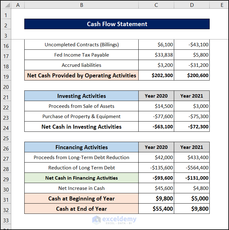
- Select the cell again and click and drag it to the right to get the value for the next year.
Download the Practice Workbook
Related Articles
<< Go Back to Financial Statement | Finance Template | Excel Templates
Get FREE Advanced Excel Exercises with Solutions!

CAN YOU PLEASE CREATE EXCEL INCOME AND BALANCE SHEETS FOR ME ME AND TELL ME YOUR PRICE.
Hello Arthur,
Thank you for your interest. If you’d like a ready-to-use template, you might check out ExcelDemy’s downloadable resources or explore freelance platforms where experts can create one tailored to your requirements.
Income and Expenditure Account and Balance Sheet Format in Excel
Excel Balance Sheet Template
Regards,
ExcelDemy