Reversing the order simply means swapping the column values. Therefore indicates the very last item in the column should be the first value in the opposite order, the next to last ought to be the second value, and so on, with the first value in a flipped column being the first value. A horizontal position is defined as a flat or level perpendicular to the plane surface; at a correct angle to the perpendicular. In this article, we will demonstrate some different effective ways to reverse the order of columns horizontally in Excel.
3 Effective Methods to Reverse Order of Columns Horizontally in Excel
While working with Microsoft Excel, we may need to reorder or rearrange the dataset we made before. We can do this by creating the dataset again with the required order. But this work is time-consuming. Excel has some amazing features and tools and also some built-in formulas to do this work just with a few clicks.
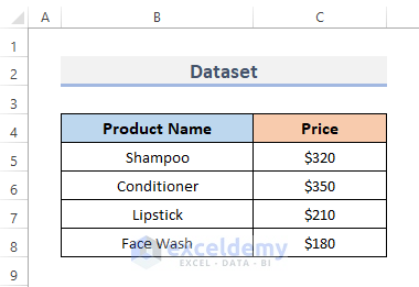
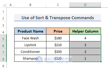
For example, we are going to use the following dataset which contains some product names and the price of the products. Now, we need to rearrange the columns by reversing them and then putting them into a horizontal order.
1. Insert Sort & Transpose Commands to Reverse Order of Columns Horizontally in Excel
Sort is a phrase used to describe the act of arranging data in a certain order to make it simpler to gather data. While sorting data in a spreadsheet, you may rearrange the data to rapidly locate data. Any or even more fields of data can be used to sort a region or list of data. Excel has the sort command to rearrange the data. We will use the sort command to reverse the data.
Transpose generates a new data source whereby the initial data document’s rows and columns are reversed. It generates new variable names instantly and provides a list of the new value labels. Excel has the transpose feature with which we will make the column in horizontal order.
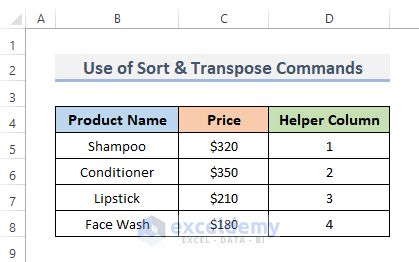
For this, we need a helper column that will help us to understand the columns are reversed.
Let’s follow the procedures to use the sort and the transpose feature in excel to reverse the order of columns horizontally.
STEPS:
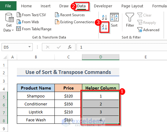
- Firstly, select the helper column to see what happens after using the sort command.
- Secondly, go to the Data tab from the ribbon of your spreadsheet.
- Thirdly, from the Sort & Filter category, click on the icon shown in the screenshot below.
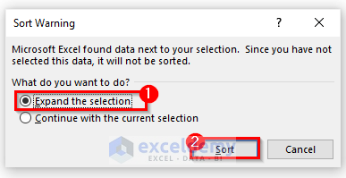
- This will open a Sort Warning dialog.
- Then, from ‘What do you want to do?‘, select Expand the selection.
- Further, click on the Sort button to sort them perfectly.
- By doing this, you can see that the columns are now just reversed.
- We don’t need the helper column anymore, so delete the helper column.
- Now, select the whole dataset and copy them by pressing the Ctrl + C keyboard shortcut.
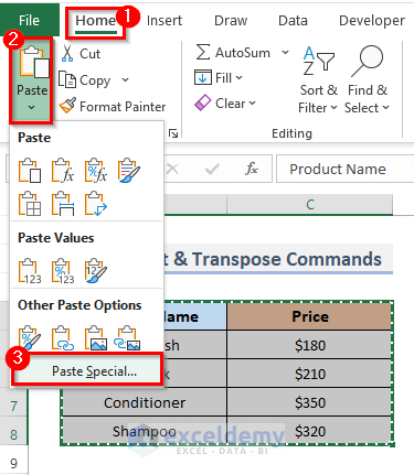
- Then, go to the Home tab of the ribbon.
- From the Clipboard category, click on the Paste drop-down menu.
- And, select Paste Special.
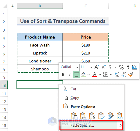
- Alternatively, you can right-click on the selected cell where you want to put the horizontal reverse order columns, and select Paste Special.
- Instead of doing this, simply you can use the keyboard shortcut Ctrl + Alt + V to open the Paste Special dialog.
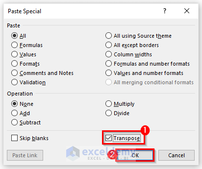
- This will display the Paste Special dialog box.
- Now, checkmark the Transpose box and click on the OK button to complete the process.
- Or, you can just click on the icon shown in the screenshot to make the columns in horizontal order.

- And, finally, you can see your desired order. By just following the above steps you can reverse the column’s order horizontally.
Read More: How to Transpose Rows to Columns in Excel
2. Reverse Order of Columns Horizontally with Excel Functions
We can use excel built-in functions to rearrange the dataset in reverse order of columns horizontally. We will see two different approaches with the formula.
2.1. Apply INDEX & TRANSPOSE Functions
First, we will use the combination of INDEX, ROWS, and COLUMNS functions to reverse the columns. The INDEX function gives the result or references to a result from a table or range of values. The ROWS and the COLUMNS function are lookup/reference functions in Excel. Then, we will use the TRANSPOSE function, a vertical range of cells is returned as a horizontal range by this function. Let’s look at the procedures to use the formulas.
STEPS:
- In the first place, we will duplicate the columns beside the original columns keeping the cell value blank to see if the formula works properly.
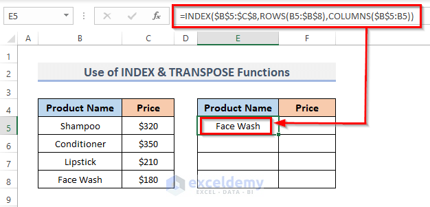
- Then, select cell E5 and put the following formula into that cell.
=INDEX($B$5:$C$8,ROWS(B5:$B$8),COLUMNS($B$5:B5))- Then, press Enter on the keyboard.
- Drag the Fill Handle down to duplicate the formula over the range. Or, to AutoFill the range, double-click on the Plus (+) symbol.
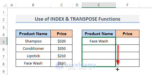
- Further, to replicate the formula throughout the range, drag the Fill Handle rightwards.

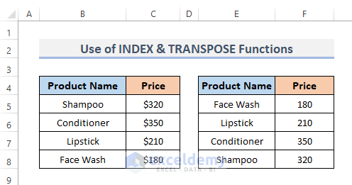
- And, finally, you will be able to see that the columns are now reversed.
🔎 How Does the Formula Work?
- COLUMNS($B$5:B5): Search up and return the column number of a specified cell reference.
- ROWS(B5:$B$8): Looks up and returns the number of rows in each reference or array.
- INDEX($B$5:$C$8,ROWS(B5:$B$8),COLUMNS($B$5:B5)): This will take the whole range of data and then reverse the columns.
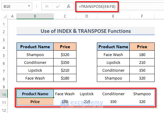
- Now, we need to set the columns in horizontal order. For this, select a cell where you want to reorder the dataset.
- Then, substitute the formula.
=TRANSPOSE(E4:F8)- Press Enter. And the formula will show in the formula bar.
- Lastly, you got the resulting order.
2.1. Use SORTBY & TRANSPOSE Functions
Second, we will combine the SORTBY function and the ROWS function to get the reverse order of columns. The SORTBY function sorts the elements of a region or an array using a formula and elements from another region or range. Then, we will use the TRANSPOSE function again to make the columns in horizontal order. Let’s follow the steps below.
STEPS:
- Likewise, in the previous methods, copy the columns without value to compare the columns.
- After that, enter the following formula there.
=SORTBY($B$5:$C$8,ROW(B5:B8),-1)- Further, to complete the operation hit the Enter key.

🔎 How Does the Formula Work?
- ROW(B5:B8): This will check and take the number of rows in each reference or array.
- SORTBY($B$5:$C$8,ROW(B5:B8),-1): Sort the range by reversing them all, -1 will put the result in the whole range of cells.
- You can now see that the columns are now in reverse order.
- Further, to make the data in horizontal order, type in the formula below.
=TRANSPOSE(E4:F8)- After that, hit Enter to see the result.
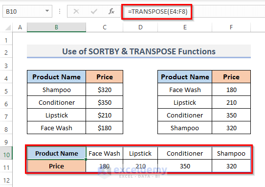
- And, that’s it. You can see the desired result on your spreadsheet.
Read More: How to Transpose Columns to Rows In Excel
3. Apply VBA Macro to Reverse Order of Columns Horizontally in Excel
With Excel VBA, users can easily use the code which acts as excel menus from the ribbon. We can use the Excel VBA to reverse the order of columns horizontally by just writing a simple code. Let’s look at the steps for using the VBA code to do the work properly. For this, we are using the same dataset as before.

STEPS:
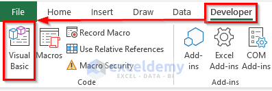
- Firstly, go to the Developer tab from the ribbon.
- Secondly, from the Code category, click on Visual Basic to open the Visual Basic Editor. Or press Alt + F11 to open the Visual Basic Editor.
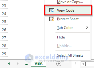
- Instead of doing this, you can just right-click on your worksheet and go to View Code. This will also take you to Visual Basic Editor.
- This will appear in the Visual Basic Editor where we write our code to create a table from a range.
- Next, copy and paste the VBA code shown below.
VBA Code:
Sub Reverse_Columns_Horizontally()
    Dim ran As Range
    Dim ary As Variant
    Dim int1 As Integer, int2 As Integer, int3 As Integer
    On Error Resume Next
    xTitleId = "Reverse Columns"
    Set ran = Application.Selection
    Set ran = Application.InputBox("Range", xTitleId, ran.Address, Type:=8)
    ary = ran.Formula
    Application.ScreenUpdating = False
    Application.Calculation = xlCalculationManual
    For int2 = 1 To UBound(ary, 2)
        int3 = UBound(ary, 1)
            For int1 = 1 To UBound(ary, 1) / 2
                xTemp = ary(int1, int2)
                ary(int1, int2) = ary(int3, int2)
                ary(int3, int2) = xTemp
                int3 = int3 - 1
            Next
    Next
    ran.Formula = ary
    Application.ScreenUpdating = True
    Application.Calculation = xlCalculationAutomatic
Range("B10:F11").Value = WorksheetFunction.Transpose(Range("B4:C8"))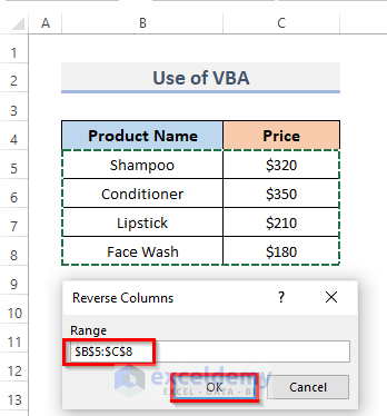
End Sub- After that, run the code by clicking on the RubSub button or pressing the keyboard shortcut F5.
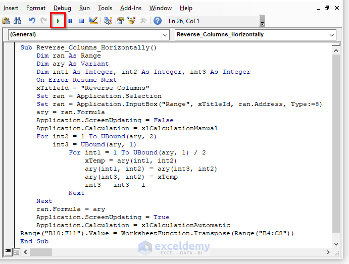
- This will appear in a window that we made by writing some code lines. The window will ask for the ranges. Select the ranges, then click OK to complete the procedure.
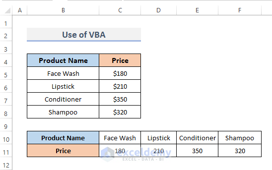
- And, you can see that the dataset columns are now in a reversed horizontal order.
VBA Code Explanation
Sub Reverse_Columns_Horizontally()
    Dim ran As Range
    Dim ary As Variant
    Dim int1 As Integer, int2 As Integer, int3 As Integer
Here, we start the procedure and name the procedure Reverse_Columns_Horizontally. Then, just declare the variable names which we need to execute the code.
xTitleId = "Reverse Columns"
    Set ran = Application.Selection
    Set ran = Application.InputBox("Range", xTitleId, ran.Address, Type:=8)
    ary = ran.Formula
    Application.ScreenUpdating = False
    Application.Calculation = xlCalculationManual
Those lines are making the window, which will ask for the ranges that we want to reverse. There we define the title box as Reverse Columns and the box name as Range.
For int2 = 1 To UBound(ary, 2)
        int3 = UBound(ary, 1)
            For int1 = 1 To UBound(ary, 1) / 2
                xTemp = ary(int1, int2)
                ary(int1, int2) = ary(int3, int2)
                ary(int3, int2) = xTemp
                int3 = int3 - 1
            Next
    Next
    ran.Formula = ary
    Application.ScreenUpdating = True
    Application.Calculation = xlCalculationAutomatic
This block of code is reversing the columns.
Range("B10:F11").Value = WorksheetFunction.Transpose(Range("B4:C8"))The line of code is making the columns in horizontal order.
Read More: VBA to Transpose Multiple Columns into Rows in Excel
Download Practice Workbook
You can download the workbook and practice with them.
Conclusion
The above methods will assist you to Reverse the Order of Columns Horizontally in Excel. Hope this will help you! If you have any questions, suggestions, or feedback, please let us know in the comment section.
Related Articles
- How to Transpose Duplicate Rows to Columns in Excel
- How to Transpose Every n Rows to Columns in Excel
- Excel VBA: Transpose Multiple Rows in Group to Columns
- Convert Columns to Rows in Excel Using Power Query
- How to Convert Columns to Rows in Excel Based On Cell Value
- VBA to Transpose Multiple Columns into Rows in Excel
- How to Convert Column to Comma Separated List With Single Quotes

