Basics of Percentage (%)
Percentage (%) is one of the most important mathematical concepts that we use in our daily lives. The percentage is level playing ground. On the basis of this ground, we compare every performance.
Every fraction can be converted to a percentage by multiplying the fraction with 100%.
100% = 100 x (1/100); [% = 1/100] = 1We can multiply any value by 1, so we can multiply any value or fraction by 100% as 100% is actually 1.
An Example
Suppose you bought a stock at $63 and sold it at $89. How much did you gain from this stock?
($89 - $63)/$63 = $26/$63 = 0.4127 = 0.4127 x 100% = 41.27%In our above example, our dollar gain was:
$89 - $63 = $26When we compare this gain ($26) with our base value $63, our gain ratio is:
$26/$63 = 0.4127To convert this fraction (or ratio) to a percentage, we have multiplied it by 100%
0.4127 = 0.4127 x 100% = 41.27%How to Calculate Percentage in Excel
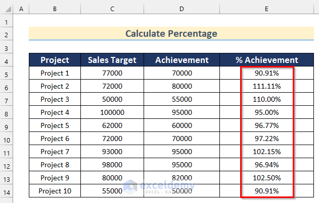
Steps:
- Select the cell range E5:E14.
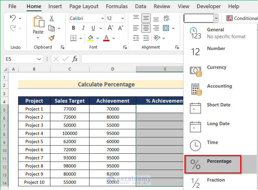
- Go to the Home tab and click on Number Format.
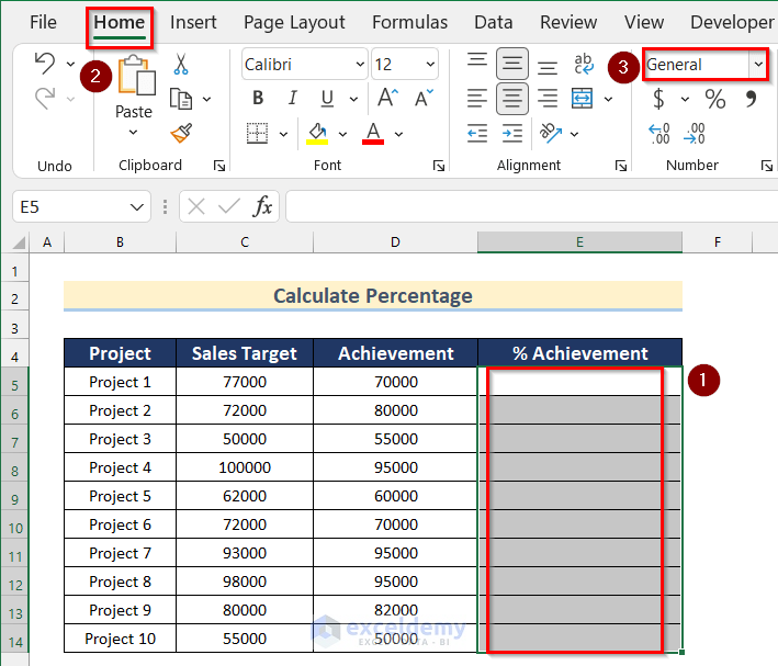
- Change the format to percentage.
You can also use the keyboard shortcut Ctrl + Shift + % to change the Format.
- Select the cell E5.
- Insert the following formula.
=D5/C5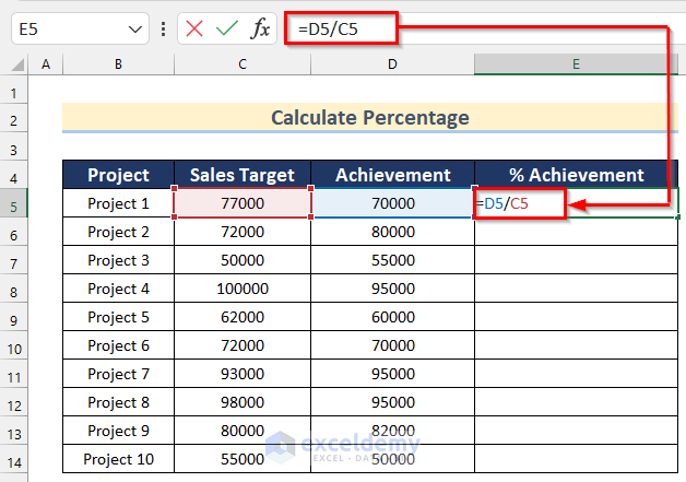
- Hit Enter and copy the formula for other cells (E5:E14) in the column.
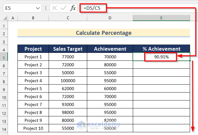
- You can increase or decrease the decimal points using two commands in the same group (Home -> Number): Increase Decimal and Decrease Decimal.
How to Use Excel Formula to Calculate a Percentage of the Grand Total: 4 Ways
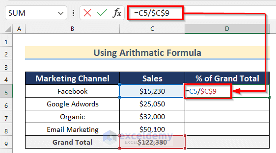
Method 1 – Using an Arithmetic Formula to Calculate a Percentage of the Grand Total for Non-Repetitive Items
We’ll use an example of a digital company that generates sales in more than one way.
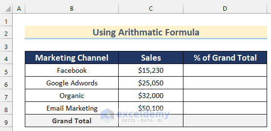
Steps:
- Select the cell C9.
- Insert the following formula.
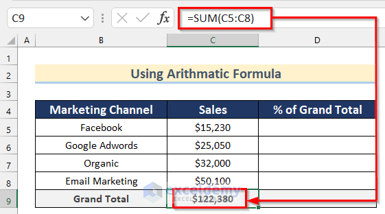
=SUM(C5:C8)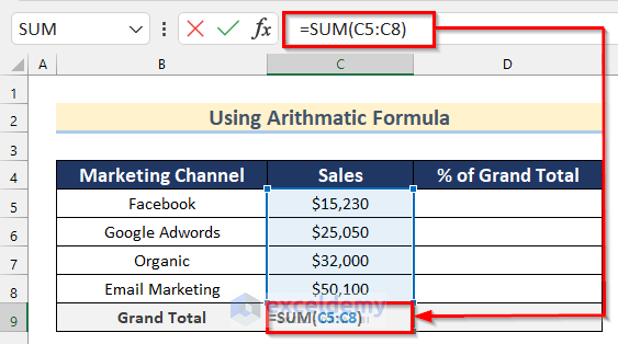
- Press Enter to get the value of the Grand Total of Sales.
- Change the Format of the cell range D5:D8 to Percentage.
- Select the cell D5.
- Insert the following formula.
=C5/$C$9The reference to C9 is fixed since we’ll copy the formula below and don’t want it to change.
- Press Enter.
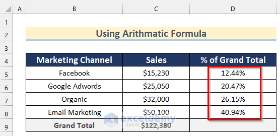
- Drag down the Fill Handle tool to AutoFill the formula for the rest of the cells.
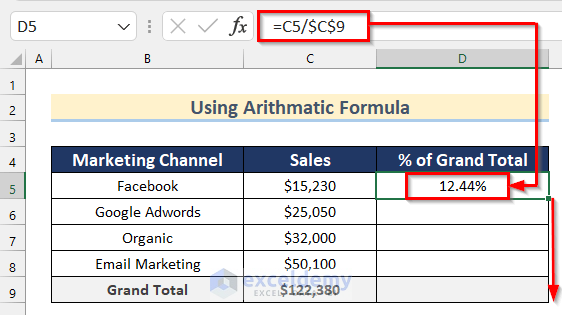
- Here’s the result.
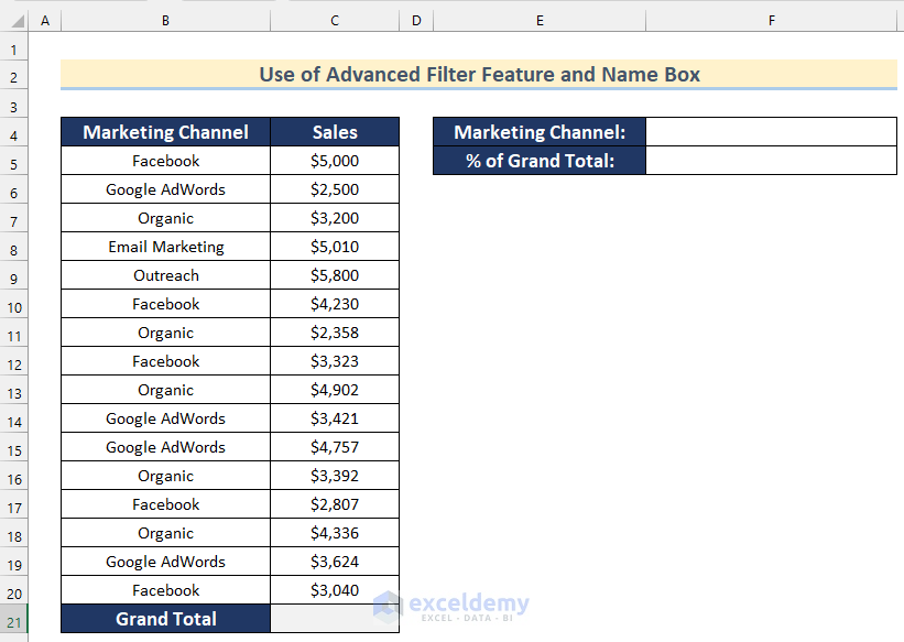
Method 2 – Using the Advanced Filter Feature and a Name Box to Calculate Percentages of the Grand Total for Repetitive Items
The marketing channels are repeated in the column. For example, Facebook has repeated 5 times, Google AdWords has repeated 4 times, and so on. At the end of the column, we need the total sales from all the channels.
Step 1 – Calculating the Grand Total to Calculate Percentage of Grand Total
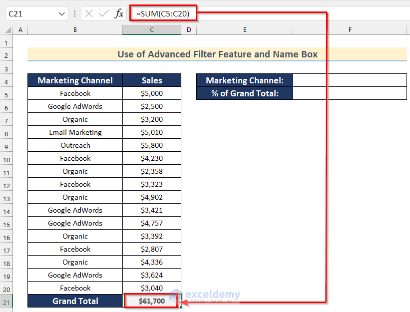
- In Cell C21, insert the following formula.
=SUM(C5:C20)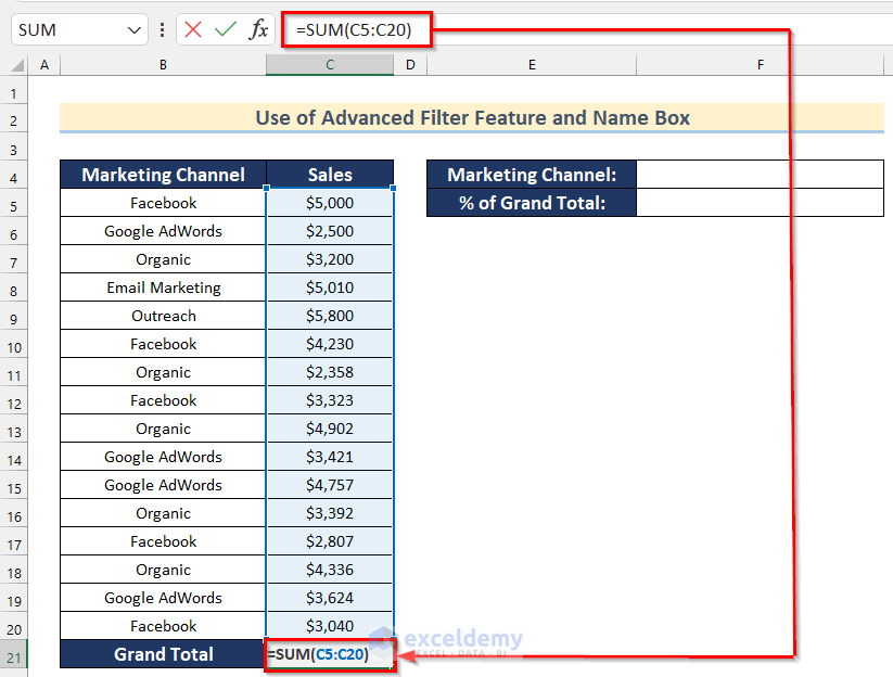
- Hit Enter to get the value of the total sales.
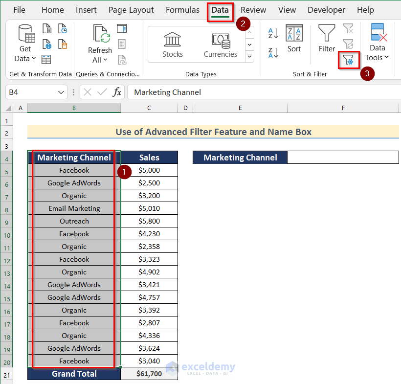
Step 2 – Finding Unique Records in Column
- Select the cell range B4:B20.
- Go to Data and click on the Advanced command in the Sort & Filter group of commands.
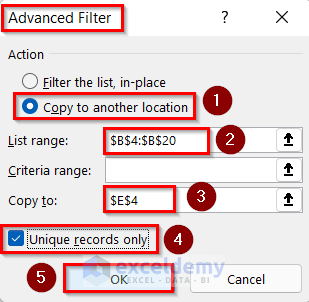
- The Advanced Filter dialog box will appear.
- Choose Copy to another location option.
- In the List range field, range $B$4:$B$20 is already set.
- In the Copy to field, input a cell where you want to place the unique records (we will choose E4).
- Check Unique records only.
- Click on OK.
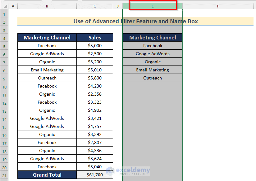
- Here’s the filtered table.

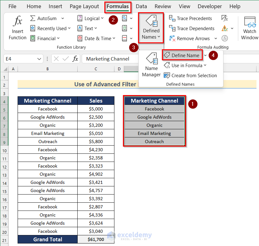
Step 3 – Making a Named Range with Unique Records
- Select the unique records (created in step 2).
- Open the Formulas ribbon.
- Click on the Define Name command in the Defined Names group of commands.
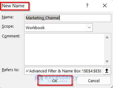
- The New Name dialog box will appear. Keep the options as-is.
- Put a name in Name.
- Click on OK.
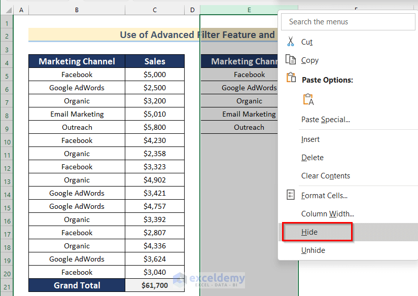
Step 4 – Hiding the Unique Records Column (Optional)
- Select Column E and right-click on it.
- Click on Hide.
Step 5 – Making a Drop-Down List with Unique Records
- Select cell G4.
- Go to Data and click on the Data Validation command from the Data Tools group.
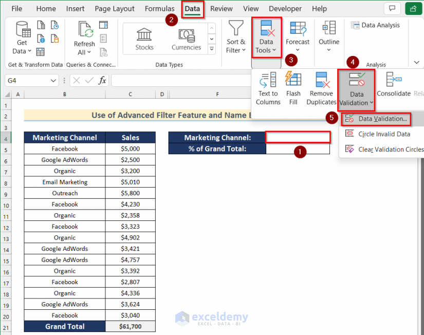
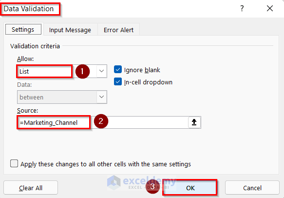
- The Data Validation dialog box appears.
- From the Allow drop-down, select the List option.
- In the Source field, input this formula:
=Marketing_Channel- Click on OK.
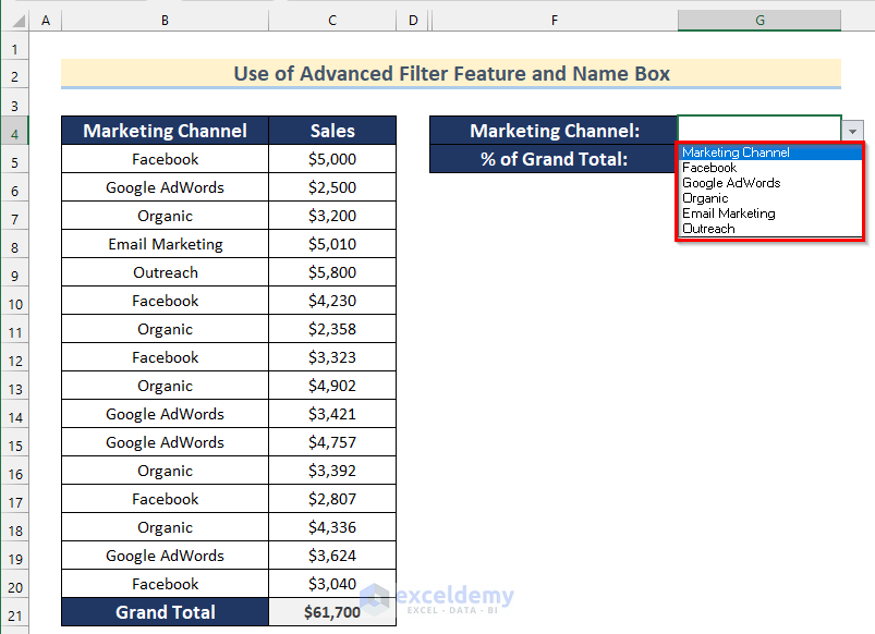
- A drop-down has been created.
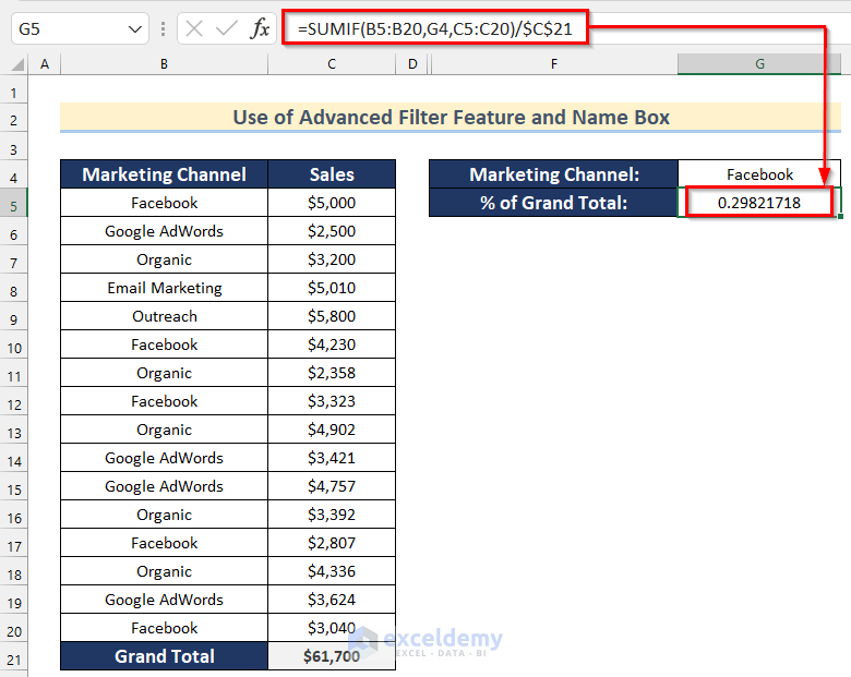
Step 6 – Calculating a Percentage of the Grand Total
- Select cell G5.
- Insert the following formula.
=SUMIF(B5:B20,F4,C5:C20)/$C$21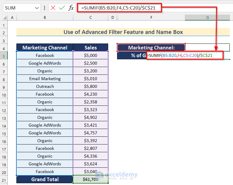
We have calculated the total sales using the Facebook channel and divided it by the Grand Total:
=SUMIF (range, criteria, sum_range) / Grand TotalThe SUMIF Function adds the cells specified by a given condition or criteria. In our example, the range is B5:B20, the criterion is the Cell reference F4 and the sum range is C5:C20.
- If we select Facebook in cell G4, we will get the ratio of Facebook and the Grand Total in cell G5.
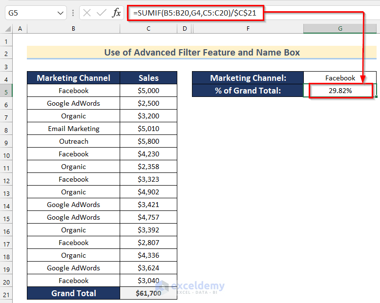
- Select Cell G5.
- Change the format to Percentage.
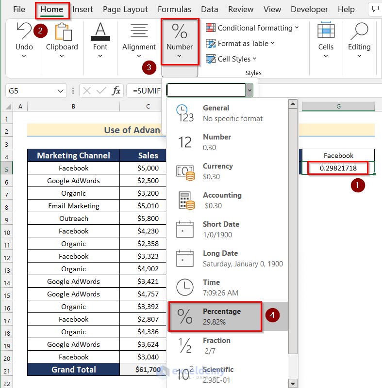
- Here’s the result.
Method 3 – Using an Excel Table to Calculate a Percentage of the Grand Total in Excel
Step 1 – Converting the Range into a Table
- Select the cell range B4:D8.
- In the Insert tab, click on the Table command.
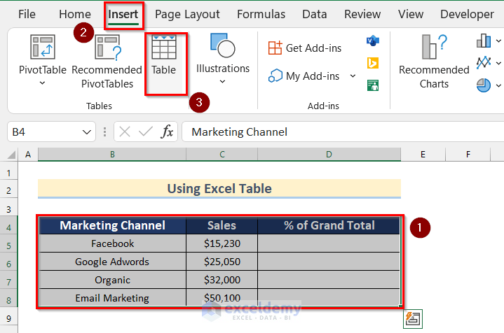
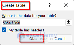
- The Create Table dialog box will appear.
- Keep the options as-is and click on OK.
- Your table will be created.
- Choose the Total Row option from the Design tab. The design tab appears only when a cell in the table is selected.
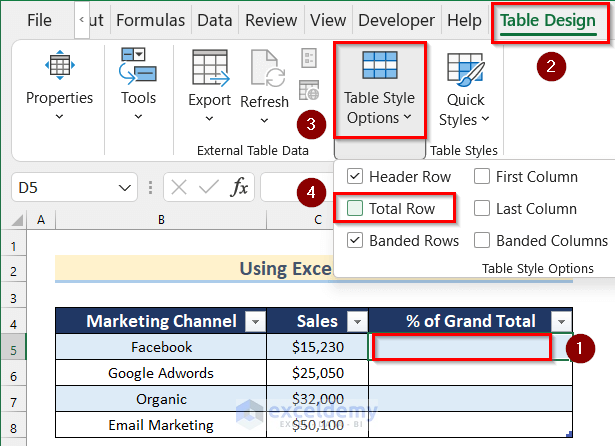
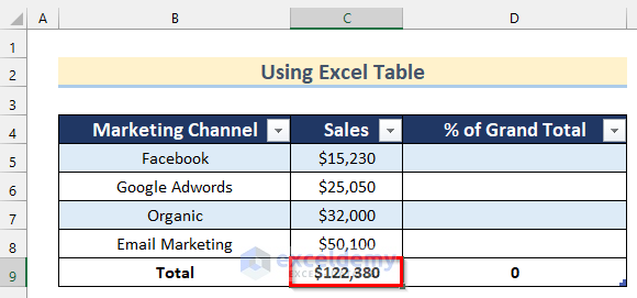
- This shows the total values under the column.
- Here is what we get.
Step 2 – Calculating a Percentage of the Grand Total
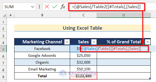
- Select the first cell (D5) of the % of Grand Total column.
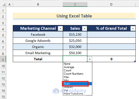
- Input an equal sign (=) and select the first cell (C5) of the Sales column.
- Input the division symbol (/).
- Select the Total cell (C9) of the Sales column.
- Press Enter.
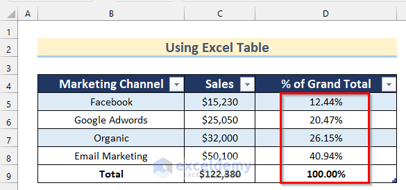
- This is what we get after applying the Percent Style in the column % of Grand Total.
Important: Benefits of using a Table instead of using a range
Adding a new row is easy in a table. Select the last cell in the table (excluding the total row) and press the Tab key on your keyboard. A new row will be created with the formula.
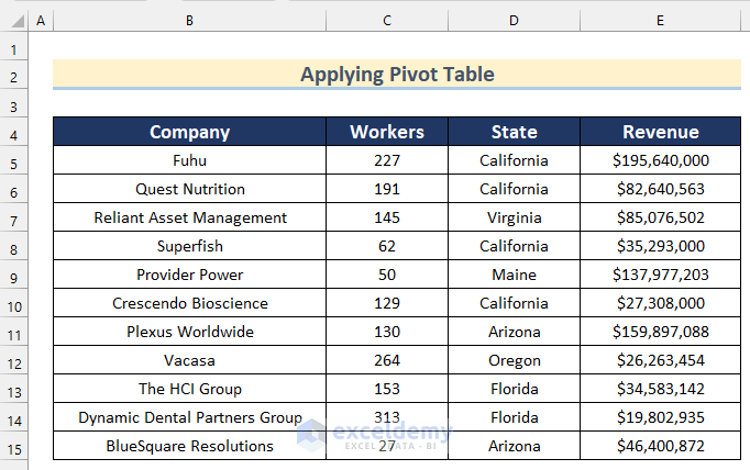
Method 4 – Inserting a Pivot Table to Calculate a Percentage of the Grand Total in Excel
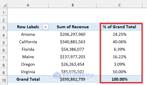
We have some data of some Company, Workers, State, and their Revenue. We will calculate the percentage of the grand total in the Excel pivot table using this dataset.
Step 1 – Creating a Pivot Table
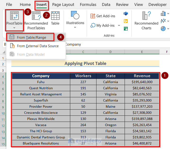
- Select the range B4:E15.
- Open the Insert tab, click on PivotTable, and select From Table/Range.
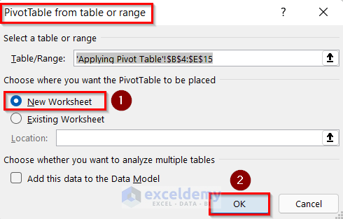
- The PivotTable from table or range dialog box appears.
- Keep the options as they are and click on OK.
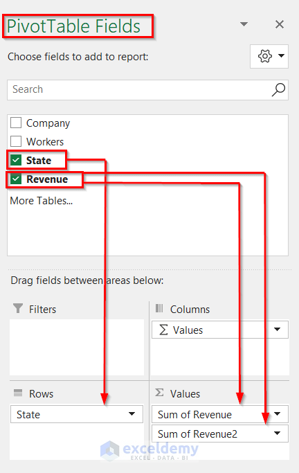
- Arrange the Pivot Table fields in the following way (image below). We have placed the Revenue field two times in the Values.
Step 2 – Calculating a Percentage of the Grand Total
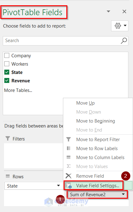
- Click on the Sum of Revenue2 field in the Values. A drop-down menu will appear.
- Click on the Value Field Setting option from the menu.
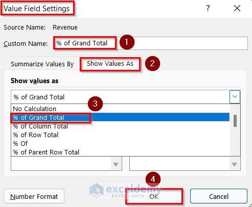
- The Value Field Settings dialog box will appear.
- Change the Custom Name field as % of Grand Total.
- Choose the Show Values As tab.
- Select the option % of Grand Total from the Show values as drop-down.
- Click on OK.
- You will see the Percentage (%) of Grand Total in the pivot table.
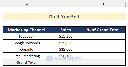
Practice Section
In this section, we are giving you the dataset to practice on your own and learn to use these explained methods.
Download the Practice Workbook
Related Articles
- Excel Formula to Add Percentage Markup
- How to Do Sum of Percentages in Excel
- How to Add Percentage to Price with Excel Formula
- How to Find the Percentage of Two Numbers in Excel
- How to Add 20 Percent to a Price in Excel
- How to Subtract a Percentage in Excel
- How to Add 10 Percent to a Number in Excel
- How to Add 15 Percent to a Price in Excel
- How to Subtract a Percentage from a Price in Excel
<<Go Back to Calculating Percentages in Excel | How to Calculate in Excel | Learn Excel
Get FREE Advanced Excel Exercises with Solutions!
