Here’s an overview of using an Excel formula to add Markup %.
Basic Formula to Add a Percentage Markup in Excel
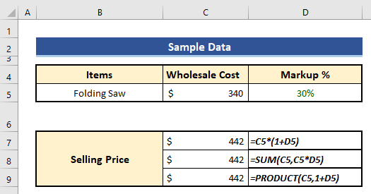
Markup is the difference between the Selling Price and the Wholesale or Production Cost of a product.
You will get the Markup % by dividing the (Selling Price – Unit Cost) by the Cost Price, multiplied by 100.

An Example to Add Percentage Markup to Cost Price:
The wholesale price (Cost Price) of a product is $25. The goal is to have a 40% Markup to the wholesale price of the product. What is the required selling price?
Selling Price = Wholesale Price x (1+Markup %) = $25 x (1 + 40%) = $25 x 1.40
Excel Formula to Add Percentage Markup – 3 Examples
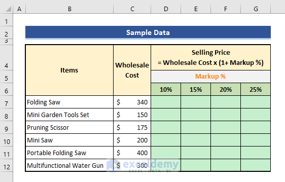
We have a list of products and want to add different Markup % to those products. Every product has a Wholesale Cost. We’ll calculate the Selling Prices of these products for different Markup Percentages (10%, 15%, 20%, 25%).
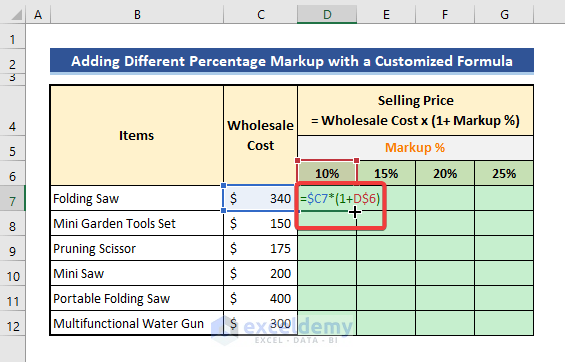
Example 1 – Use a Customized Excel Formula to Add a Markup
Steps:
- In cell D7, use the following Excel formula:
=$C7*(1+D$6)
Quick Notes:
- The formula has mixed cell references. Column C and Row 6 are made of absolute references.
- When we go down or up, row references change. When we go left or right, column references change.
- When filling to the right, $C will not change to keep the wholesale cost reference intact.
- When copying the formula down, the row references $6 will not change to get the correct Markup % reference.
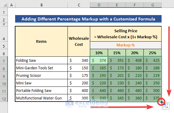
- Pull the Fill Handle icon to the right and then down.
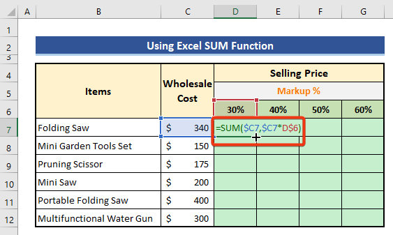
Example 2 – Apply the Excel SUM Function to Add a Percentage Markup
Steps:
- Put the formula below in Cell D7.
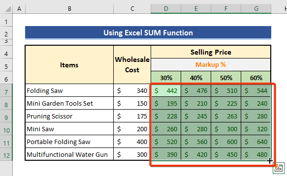
=SUM($C7,$C7*D$6)
- Drag the Fill Handle icon right, then down.
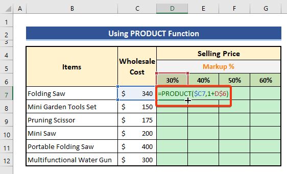
Example 3 – Use the PRODUCT Function
The PRODUCT function multiplies all numbers given as arguments.
Steps:
- Go to Cell D7 and paste the following formula.
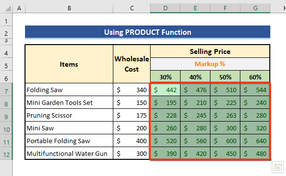
=PRODUCT($C7,1+D$6)
- Pull the Fill Handle icon to reach G12.
Download the Practice Workbook
You can use the downloaded file as a calculator.
Related Articles
- How to Do Sum of Percentages in Excel
- How to Add Percentage to Price with Excel Formula
- How to Add 20 Percent to a Price in Excel
- How to Subtract a Percentage in Excel
- How to Use Excel Formula to Calculate Percentage of Grand Total
- How to Add 10 Percent to a Number in Excel
- How to Add 15 Percent to a Price in Excel
- How to Subtract a Percentage from a Price in Excel
<< Go Back to Add Percentage to a Number in Excel | Calculating Percentages in Excel | How to Calculate in Excel | Learn Excel
Get FREE Advanced Excel Exercises with Solutions!

Hello, thank you fr the post, really helpful insights, but what if your product cost varies, for instance when importing, is there any way to create a formula to determine the margin when there is an increase or decrease? I’m struggling to get that one right