Looking for ways to know how to create a bubble chart in Excel with labels? Usually, we use bubble charts to graphically visualize multiple numerical variables. Here, you will find step-by-step explained ways to create a bubble chart in Excel with labels.
How to Create a Bubble Chart in Excel with Labels: 4 Effective Ways
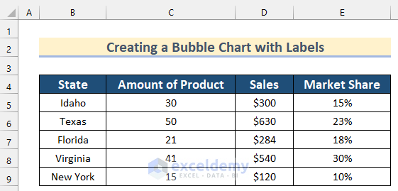
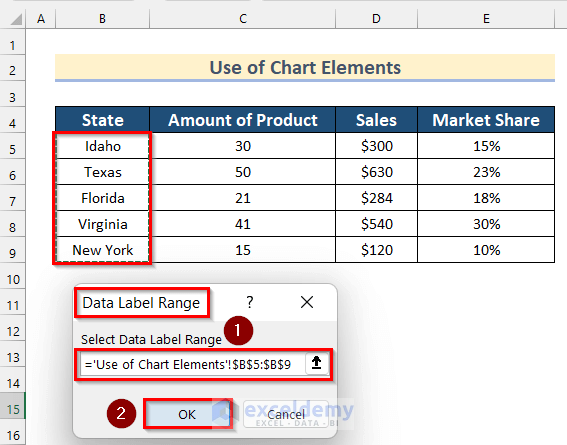
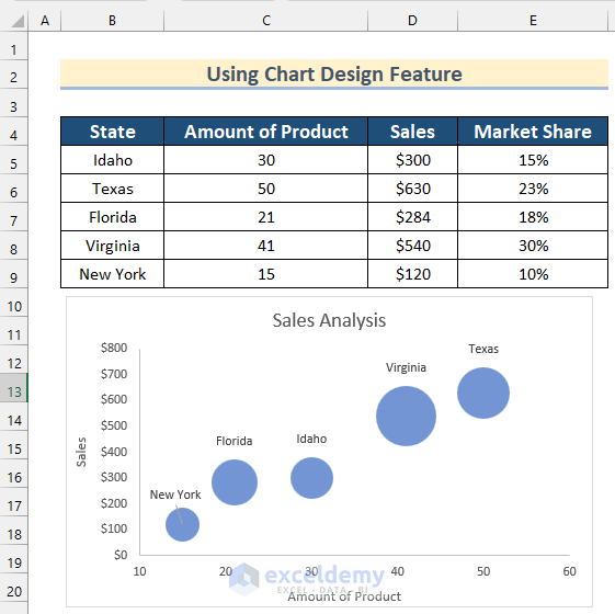
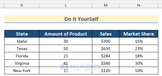
Here, we have a dataset containing the data of State, Amount of Product, Sales, and Market Share of a shop. Now, we will use this dataset to show you how to create a bubble chart in Excel with labels.
1. Use of Chart Elements to Create a Bubble Chart with Labels
In the first method, we will show you how to create a bubble chart with labels in Excel using Chart Elements. Go through the steps given below to do it on your own dataset.
Steps:
- First, select Cell range C5:E9.
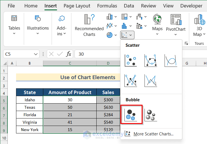
- Then, go to the Insert tab >> click on Scatter or Bubble Chart.
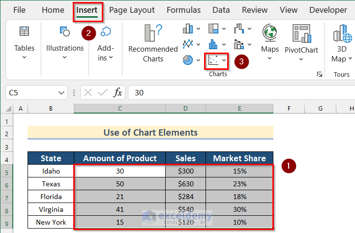
- After that, select the Bubble chart.
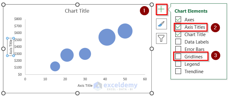
- Now, you will see a Bubble Chart with the Amount of Product as X-axis, Sales as Y-axis, and Market Share as the size of the Bubble.
- Next, click on the “+” sign to open Chart Elements.
- Then, turn on Axis Titles and turn off Gridlines.
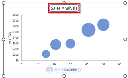
- Afterward, click on the Chart Title to change it.

- Now, type “Sales Analysis” as Chart Title.
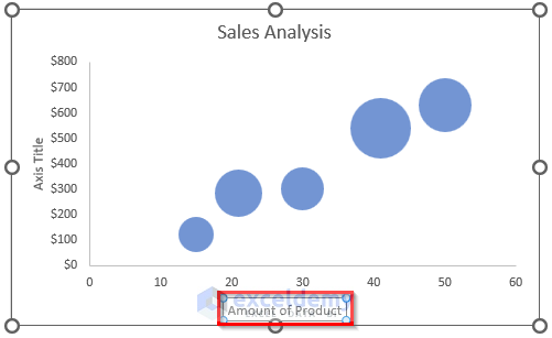
- After that, click on the Axis Title of the X-axis.

- Then, type “Amount of Product” as Axis Title.
- Next, click on the Axis Title of Y-axis.
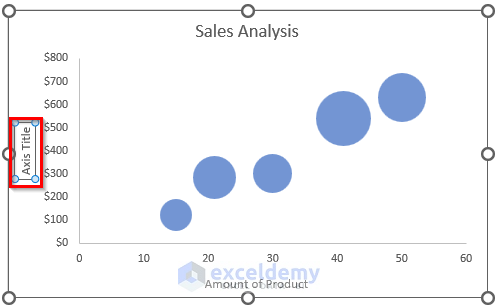
- Afterward, type “Sales” as Axis Title.

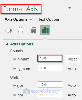
- Now, double-click on the X-axis.

- After that, the Format Axis toolbar will open.
- Then, change the Minimum bounds as 10.
- Finally, you will get your Bubble Chart with Chart Title and Axis Titles.

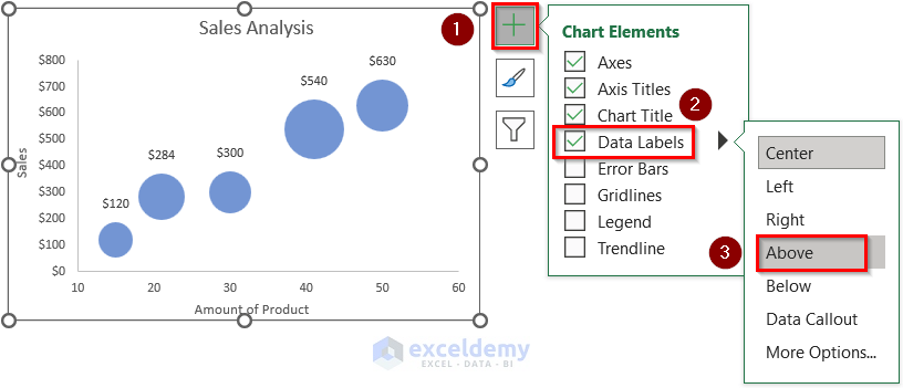
- Then, click on the “+” sign to open Chart Elements.
- After that, turn on Data Labels >> click on More Options.

- Now, the Format Data Labels toolbar will appear.
- Next, from Label Options select Above as Label Position.
- Then, select Value From Cells in Label Contains.

- After that, the Data Label Range box will open.
- Next, select Cell range B5:B9 in the Select Data Label Range box.
- Now, press OK.
- Again, from the Label Options turn off Y Value.

- Thus, you will create a Bubble Chart with labels using Chart Elements.

Read More: How to Create Bubble Chart in Excel
2. Using Chart Design Feature to Create a Bubble Chart with Labels
We can also use Chart Design Feature to create a bubble chart with labels in Excel. Follow the steps given below to do it on your own.
Steps:
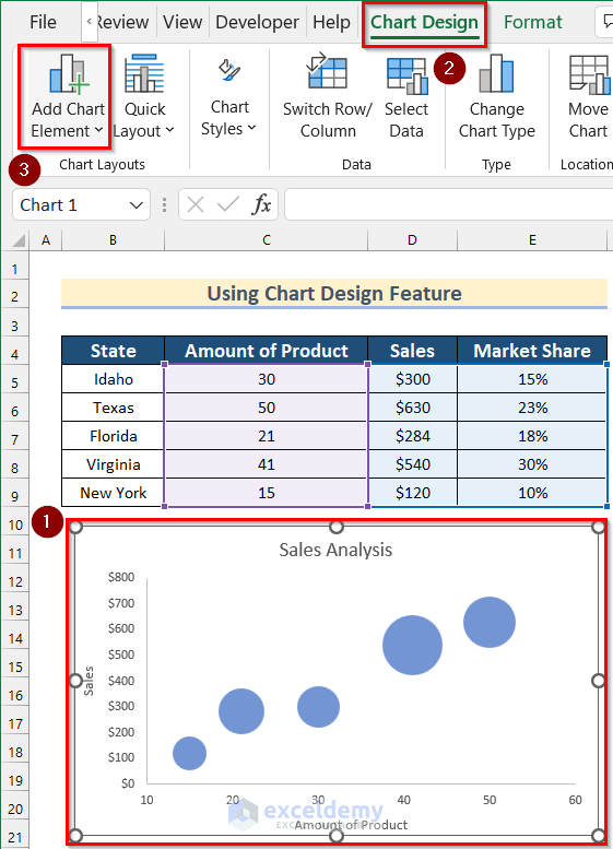
- In the beginning, create a Bubble Chart by following the same steps given in Method1.
- Then, select the Bubble Chart.
- After that, go to the Chart Design tab >> click on Add Chart Element.
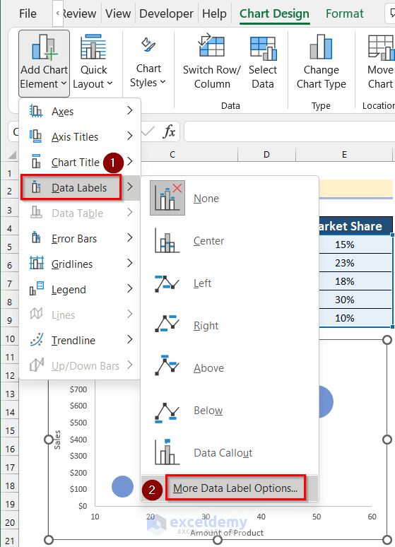
- Next, click on Data Labels >> select More Data Label Options.
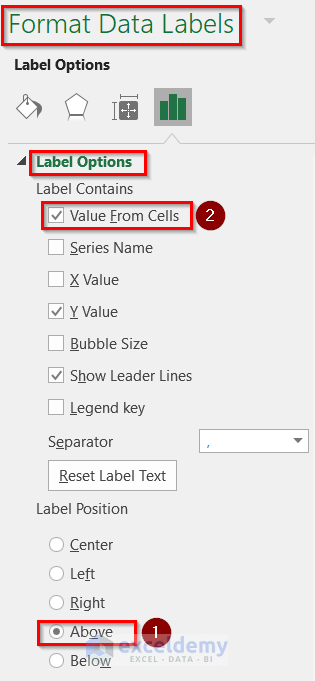
- Now, the Format Data Labels toolbox will appear.
- Next, from Label Options select Above as Label Position.
- Then, select Value From Cells in Label Contains.
- After that, the Data Label Range box will open.
- Next, select Cell range B5:B9 in the Select Data Label Range box.
- Now, press OK.

- Again, from the Label Options turn off Y Value.

- Thus, you will create a Bubble Chart with labels using Chart Design Feature.
Read More: How to Create 4 Quadrant Bubble Chart in Excel
3. Manually Changing Labels to Create a Bubble Chart with Labels in Excel
Now, we will show you how to create a bubble chart with labels by Manually Changing Labels. Go through the steps given below to do it on your own dataset.
Steps:
- First, create a Bubble Chart by following the same steps given in Method1.

- Then, click on the “+” sign to open Chart Elements.
- After that, turn on Data Labels >> select Above.
- Next, select any Data Label by clicking on it. Here, we selected $120.
- Then, insert the following formula in the Formula Bar to select Cell B9 as Data Label.
='Manually Changing Labels'!$B$9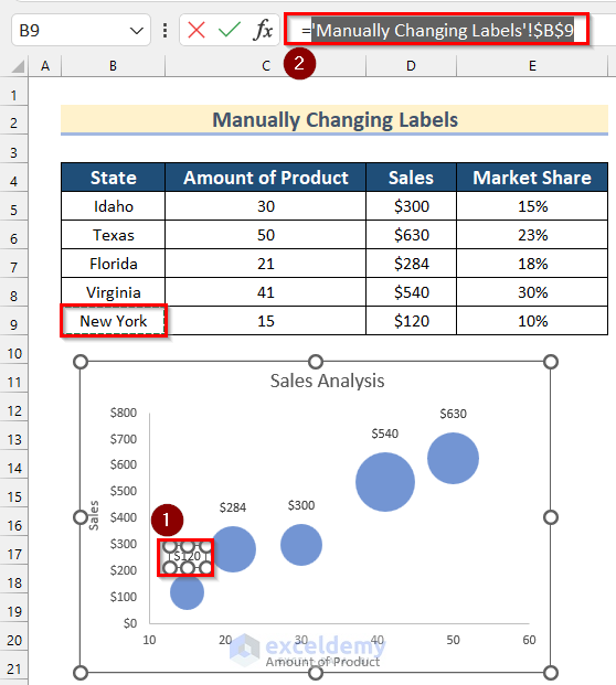
- Now, press ENTER.

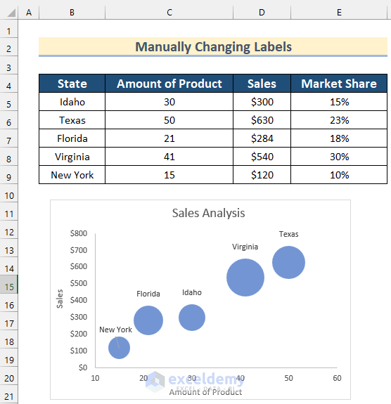
- Similarly, insert the corresponding Cell value for all the Data Labels.
- Finally, you will get your desired Bubble Chart with labels by Manually Changing Labels.
Read More: Excel Bubble Chart Examples
4. Using Text Box Feature to Create a Bubble Chart with Labels in Excel
In the final method, we will use the Text Box feature to create a bubble chart with labels in Excel. You can use the Text Box to add text anywhere in the chart.
Follow the steps given below to do it on your own.
Steps:
- In the beginning, create a Bubble Chart by following the same steps given in Method1.
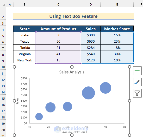
- Then, select the Bubble Chart.
- After that, go to the Insert tab >> click on Text >> select Text Box.

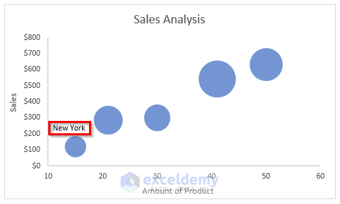
- After that, insert a Text Box anywhere in the chart and type your desired value. Here, we will add a Text Box and will type New York.
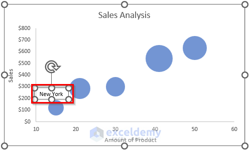
- Now, press ENTER.
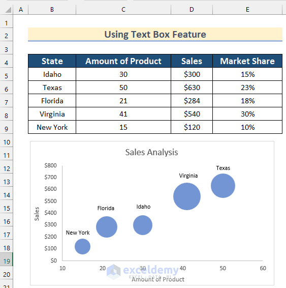
- Similarly, insert the corresponding Cell value for all the Data Labels using Text Box.
- Finally, you will get your desired Bubble Chart with labels using Text Box Feature.
Read More: How to Create a 3D Bubble Chart in Excel
Things to Remember
- To use Chart Elements, make sure you have selected the bubble chart. Otherwise, the Chart Element tab will not appear.
- Moreover, In the case of using Text Box, select the bubble chart first to move the text with the chart.
Practice Section
In this section, we are giving you the dataset to practice on your own and learn to use these methods.
Conclusion
So, in this article, you will find a step-by-step way to create a bubble chart in Excel with labels. Use any of these ways to accomplish the result in this regard. Hope you find this article helpful and informative. Feel free to comment if something seems difficult to understand. Let us know any other approaches which we might have missed here. Thank you!
Related Articles
<< Go Back To Bubble Chart in Excel | Excel Charts | Learn Excel
Get FREE Advanced Excel Exercises with Solutions!
