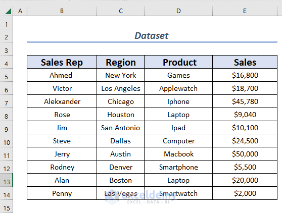
To demonstrate the different methods, we will use a dataset of sales information, consisting of the sales of particular products by different sales reps in different regions.
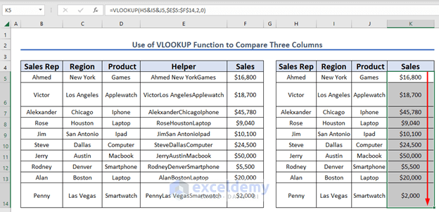
Method 1 – Use VLOOKUP Function
Steps:
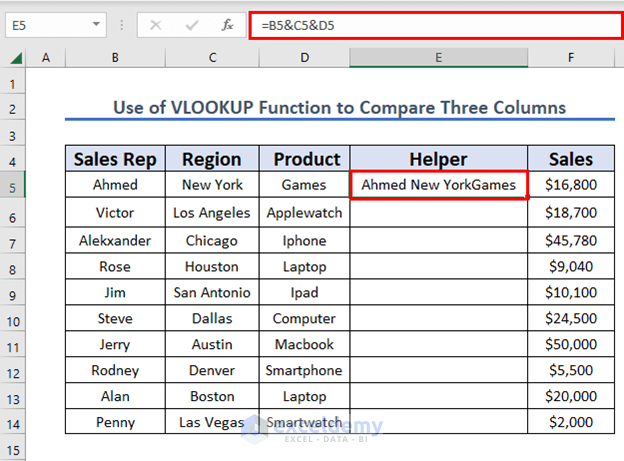
- In column E, insert a column in the dataset named “Helper”.
- In cell E5 enter the following formula
=B5&C5&D5- Press ENTER to return the output.
- Use Fill Handle to AutoFill up to cell E14.
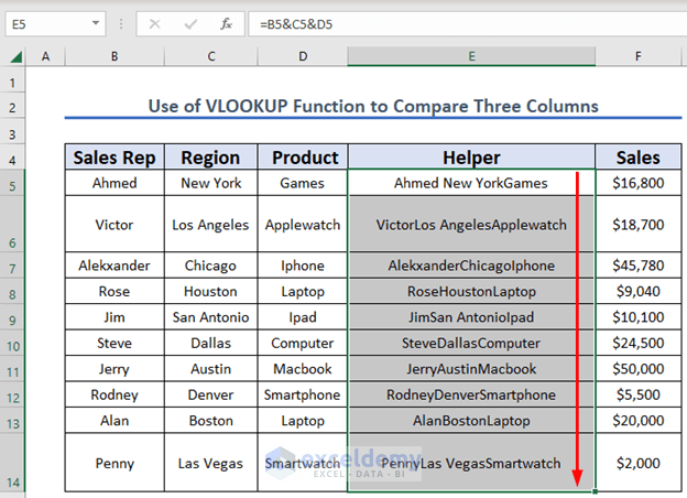
Now let’s compare the three columns Sales Rep, Region, and Product with the same columns from another table, and retrieve the Sales for matches.
Steps:
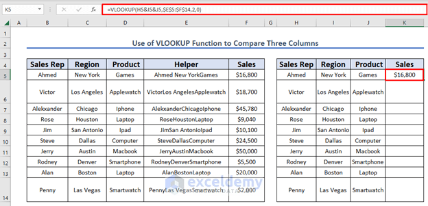
- In cell K5 enter the following formula:
=VLOOKUP(H5&I5&J5,$E$5:$F$14,2,0)- Press ENTER to return the output.
Formula Explanation
- Here, the lookup_value is H5&I5&J5.
- The table_array is $E$5:$F$14. Excel will look for H5&I5&J5 in this array.
- The col_index is 2. Excel will return the corresponding Sales.
- Use Fill Handle to AutoFill up to cell K14.
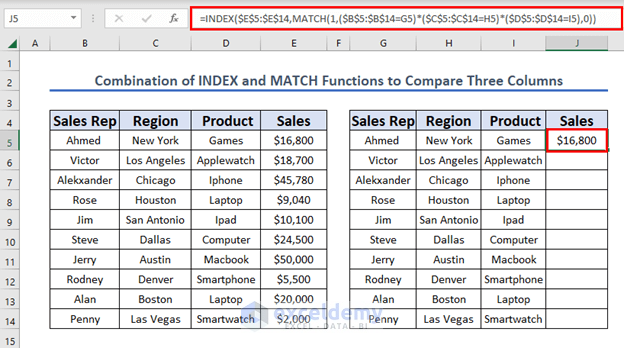
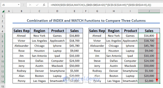
Method 2 – Combine INDEX and MATCH Functions
Steps:
- In cell J17 enter the following formula:
=INDEX($E$5:$E$14,MATCH(1,($B$5:$B$14=G5)*($C$5:$C$14=H5)*($D$5:$D$14=I5),0))- Press ENTER to return the output.
Formula Breakdown
- ($B$5:$B$14=G5)*($C$5:$C$14=H5)*($D$5:$D$14=I5) → This is the lookup_array for the MATCH function.
- Output: {1;0;0;0;0;0;0;0;0;0}
- MATCH(1,($B$5:$B$14=G5)*($C$5:$C$14=H5)*($D$5:$D$14=I5),0) → This is the row_num for the INDEX function.
- Output: 1
- INDEX($E$5:$E$14,MATCH(1,($B$5:$B$14=G5)*($C$5:$C$14=H5)*($D$5:$D$14=I5),0))
- This formula resolves to INDEX($E$5:$E$14,1)
- Output: $16,800
- Use Fill Handle to AutoFill the formula up to cell J14.
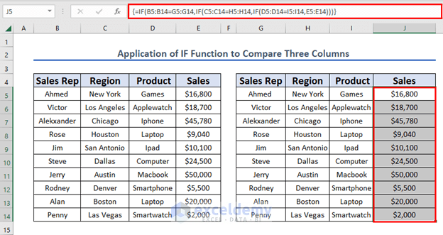
Method 3 – Use the IF Function
Steps:
- In cell J5 enter the following formula:
=IF(B5:B14=G5:G14,IF(C5:C14=H5:H14,IF(D5:D14=I5:I14,E5:E14)))- Press CTRL + SHIFT + ENTER to return the output. Since this is an array formula, all sales will be returned at once.
Formula Explanation
- This is a nested IF formula.
- B5:B14=G5:G14 is the logic test for the first IF function.
- Output: {TRUE;TRUE;TRUE;TRUE;TRUE;TRUE;TRUE;TRUE;TRUE;TRUE}
- Since the output is TRUE, the result will be IF(C5:C14=H5:H14,IF(D5:D14=I5:I14,E5:E14))
- The rest of the IF functions work similarly to the first one.
- Output: {16800;18700;45780;9040;10100;24500;50000;5500;20000;2000}
Note the curly bracket {} in the formula bar, which indicates an array formula.
Method 4 – Apply SUMPRODUCT Function
Steps:
- In cell J5 enter the following formula:
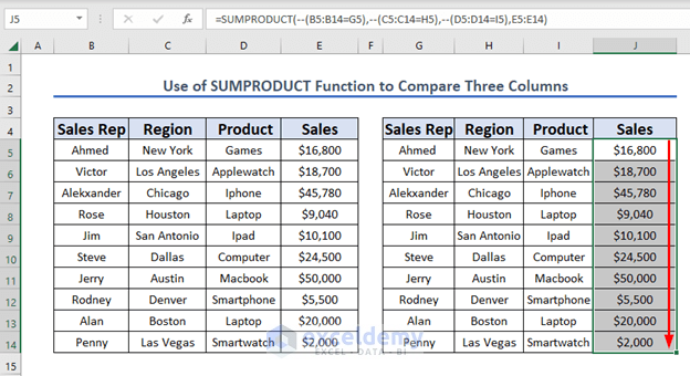
=SUMPRODUCT(--(B5:B14=G5),--(C5:C14=H5),--(D5:D14=I5),E5:E14)- Press ENTER to return the output.
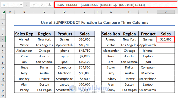
Formula Explanation
- There are four arrays in the formula.
- The output for the first three arrays is the same: {1;0;0;0;0;0;0;0;0;0}
- Hence the sum products of these arrays are the corresponding Sales.
- Use Fill Handle to AutoFill the formula up to cell J14.
Download Practice Workbook
<< Go Back to Columns | Compare | Learn Excel
Get FREE Advanced Excel Exercises with Solutions!

Hello, I have 3 columns. employee ID, date and dollars. Not all dates for each employee have dollar. I want to return dates that have dollars for each employee. How do I proceed.
Thank you
Hello Jim,
Thanks for commenting. If I am not wrong, you want to sort dates that don’t have the dollar like the dataset below.
Select the entire data range then navigate the Home tab >> choose Sort & Filter from #diting group >> pick Filter.
Choose the Filter dropdown and uncheck the blanks from the column.
Finally, the dates are sorted with the dollar.
Regards
Fahim Shahriyar Dipto
Excel & VBA Content Developer
Hello, i want to match 3 columns Customer name, ID name and Real name resp. and if both name not matched with ID name then , they should be highlighted with colour.
ex.
jenith jeneth jenath riq
Hello Chandan,
Thanks for commenting. If I’m not wrong, you want to match the dataset like the one below.
Select the entire dataset without the heading then go to conditional formatting >> New Rule
Then select “Use a formula to determine which cells to format.”
In the formula bar, enter the following formula:
=AND(A3<>B3,C3<>B3)
Press OK
Here, “A3” represents the cell containing the customer name, “B3” represents the cell containing the ID name, and “C3” represents the cell containing the real name. You can adjust the cell references based on your data.
Choose the formatting option that you want to use for the highlighted rows. For example, we took light green color here for highlighting.
The final outcome will look like the image below.
I hope this answer will help you to identify matched names. Please let us know if you have any other queries. Also, you can post your Excel-related problem in ExcelDemy Forum with images or Excel workbooks.
Regards
Mizbahul Abedin | ExcelDemy Team