Microsoft Excel has multiple ways of performing autosum in spreadsheets. In this article, we will show how to autosum time in Excel. The methods described in the article might be helpful in calculating the total working hours of employees in a month, the total time taken to complete several tasks, and so many other situations. So, let’s begin today’s journey.
This section will demonstrate 4 effective methods for Autosum in Excel. For illustration, let’s assume that we have a data table where weekly working hours for four employees of a company are given. ( See the figure below)

Now, we want to autosome the total working hours for each employee in column G. To accomplish that, let’s check our first method.
1. Using Autosum Option to Autosum Time in Excel
This is a very straightforward method. In this method, we will use the Autosum option. Follow the steps given below to know how this method works.
Steps:
- First, select all the cells of the column named Total.
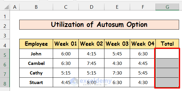
- Now, go to the Editing group in the Home tab and click on the Autosum Option icon (Shown in the figure below)

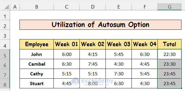
- Consequently, you will get the Sum of times for each row.
2. Applying SUM Function to Autosum Time in Excel
We can also use the SUM function in addition to the Autosum option to autosum time in Excel. To do that, follow the steps below.
Steps:
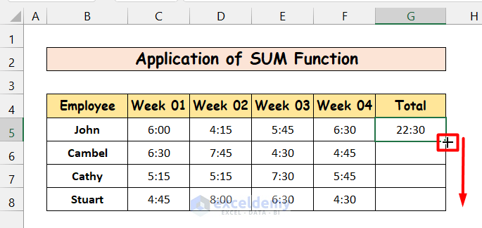
- First, click on cell G5 and write down the following formula.
=SUM(C5:F5)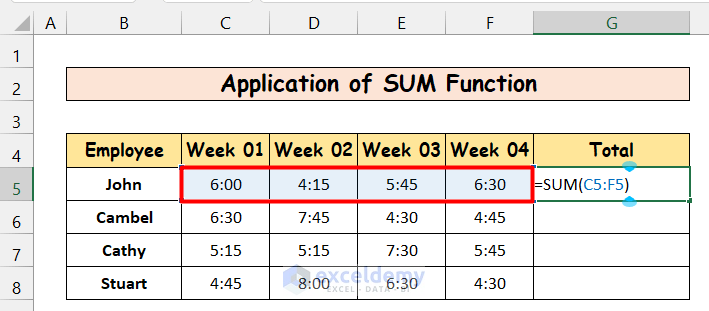
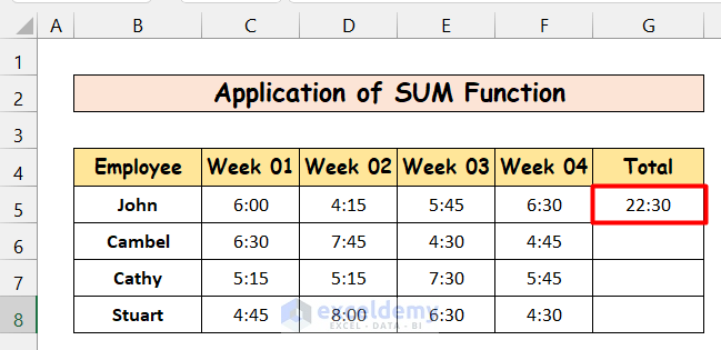
- Now, press Enter, and you will see the Sum of times of the first row.
- Then, we can use the Fill Handle to copy the formula to other cells as well.
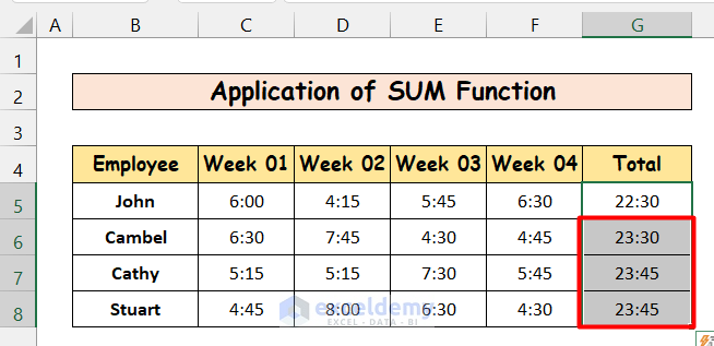
- As a result, we will get the Sum of times of all rows in the table.
3. Use a Shortcut Key to Autosum Time
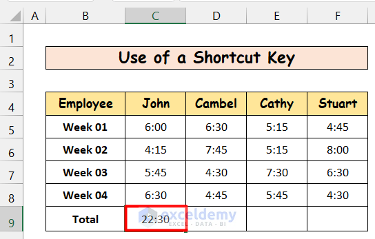
This method is not so popular but useful when we need to autosome data in a column. Hence to illustrate this method, we have to transpose the timetable like this.

Now in this arrangement, we have to autosum time in column-wise. Follow the steps below to learn how we can use a shortcut key to autosum time in excel.
Steps:
- First, select cell C9.
- Then press Alt +=
- And now click Enter You will have the following result.
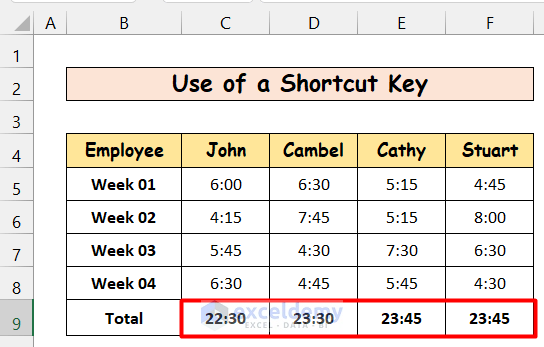
- Now, do the same thing in cells D9 to F9. The final result will be the same as the previous two methods.
Read More: How to Autosum Column in Excel
4. Use of Total Row Option to Autosum Time in Excel
This method uses the Total Row option in the Excel table to autosum time in Excel. Similar to 3rd method, the time is summed column-wise. Hence, we need to organize the dataset as shown in the figure below.
Figure 12
Now, to do autosum, follow the steps below.
Steps:
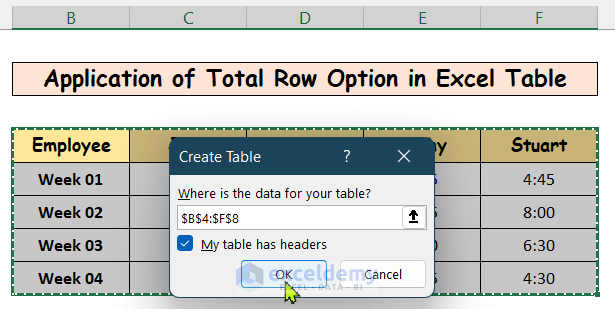
- First, we need to convert the data set into an Excel table. Select the entire data set and click on Format as Table in the Styles group. From the available table design, click on any suitable one.

- Now in the Create Table dialogue box, click on My Table has headers and then click OK.
- Now that we have created a table, we need to add Total Row. To do that, click on any table cell, go to the Table Design tab and check the Total Row Consequently, a new row will be created. (Shown in the figure below)

- Now, click on cell Then from the dropdown menu, choose Sum. You should see the Sum of times in the first column.

- Do the same tasks again to get all the desired Sum of times for the rest of the columns.

How to Sum Time Over 24 Hours in Excel
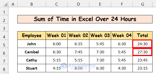
If we have a set of times whose Sum is more than 24 hours, we need to modify the format to display accurate results. ( See the figure below)

Here we can see that the cells G5 and G6, the displayed results are not what we expected. In G5 and G6, we should have got 24:30 and 27:30, respectively. This anomaly is due to the formatting of the cells. To solve the issue, follow the steps below:
Steps:
- Select the last column and go to the Number group and click on the down arrow (see the figure below)

- Then, in the Type box, write the following text [h]:mm;@

- Now, click OK. As a result, the sums will be shown in the desired format.
Things to Remember
- The first two methods are applicable for both row-wise and column-wise summing.
- The third and fourth methods are only applicable for column-wise summing.
Download Practice Workbook
Download this practice workbook to exercise while you are reading this article.
Conclusion
That is the end of this article. If you find this article helpful, please share this with your friends. Moreover, do let us know if you have any further queries.
Related Articles
- [Fixed!] Excel AutoSum Not Working
- [Solved!] Excel AutoSum Is Not Working and Returns 0
- How to Turn Off AutoSum in Excel
- How to AutoSum Horizontally in Excel
- How to Calculate Percentage Using AutoSum in Excel
<< Go Back to Autosum in Excel | Sum in Excel | Calculate in Excel | Learn Excel
Get FREE Advanced Excel Exercises with Solutions!
