Latest Posts From Alok Paul

The TAN function is in the Trigonometry Functions list under the Math and Trig Functions category that calculates the slope of a tangent of an angle of any ...

The Excel VAR function is categorized as a Statistical function of Microsoft Excel. It determines the risk of any investment and, hence, is important for ...

The FV function is a default function of Microsoft Excel which is categorized as a financial function. It helps to figure out the future value of an ...

This EFFECT function is a financial function of Microsoft Excel. It is calculated based on the nominal rate of interest and compound periods in a year. This ...

This is an overview: The ABS Function Function Objective: The ABS function is used to get the absolute value of a number. You will get ...

Introduction to the SUBTOTAL Function The SUBTOTAL function returns a list or database and falls under the Math/Trig function category. It offers 11 Excel ...

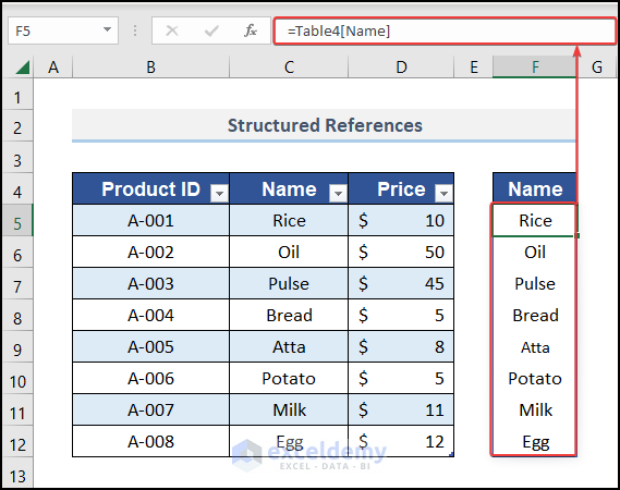
Excel INDEX Function The INDEX function returns a value or the reference to a value from within a table or range. The INDEX function is used in two ...

Method 1 - Using ISODD Function Steps: Select the column where you want to change the text color. Go to the Home tab. Select the New Rule from the ...

Method 1 - Combine IF and AND Functions to Calculate If Cells are Not Blank Step 1: Add a row to show the calculation. Step 2: Go to Cell C14. ...
In this article, we will discuss table formatting problems in Excel. We'll use a simple dataset to show solutions. Excel Table Formatting Problems: ...
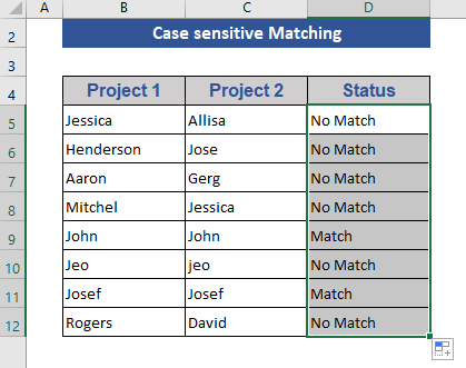
We'll use a simple dataset of employees assigned to two projects for a few of the methods. Method 1 - Combining Excel IF and EXACT Functions to Compare ...

In this article, we will demonstrate 5 easy ways to determine how many digits a number in a cell has. Why Count Numbers in a Cell in Excel? ...

In this article, we describe how to split data into multiple Excel worksheets using VBA & Macros. In our data set, we have data comprising ...

In this article, we will discuss 4 different methods to highlight blank cells in Excel. We'll use the following dataset of the names of some students in ...
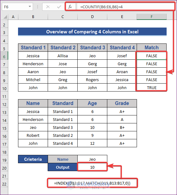
Method 1 – Using Conditional Formatting Steps: Select the cells of 4 Columns from the dataset. Go to the Home tab. Select the Conditional ...
See Our Reviews at


Dear CC,
Thank you very much for reading our articles.
You have requested an updated VBA code to retain borders as well. Please try the provided VBA code below; it preserves borders.
Best Regards,
Alok
Team ExcelDemy
Hi RED,
Thanks for reading our articles. Hope you are doing well.
You want to copy the rows of data without the header row duplicated on each worksheet.
There may be two situations:
Case 1: The header row will not exist in any of the split worksheets.
Case 2: The header row will exist on the first split worksheet.
For Case 1: Change the 13th line of the current VBA code from title = “A1” to title = “A2”. After making this adjustment and running the VBA, the header row will not be visible in the split worksheets.
For case 2: We added a variable named isFirstSheet to distinguish the first split sheet, displaying the header row, and excluding it from subsequent sheets. Employ the updated VBA code provided below:
We have marked the modified section of the VBA code in the above image.
Best Regards,
Alok
Team ExcelDemy
Hi JAD,
I hope you are doing well. Thank you very much for reading our articles.
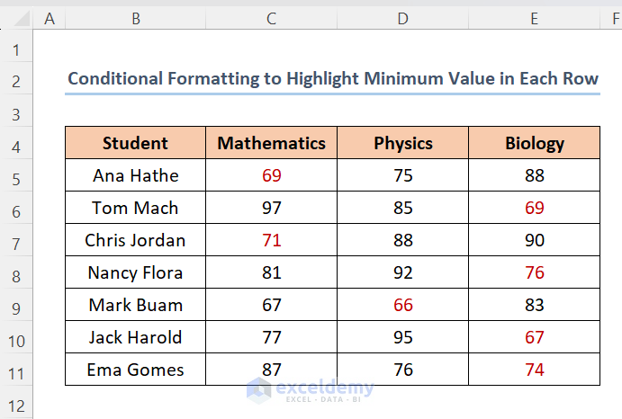
You want to apply conditional formatting to the minimum value in each row across multiple rows. For that, you need to use a formula in the conditional formatting. Follow the instructions given below:
=C5=MIN($C5:$E5)You can see minimum values of each row have been highlighted.
Regards,
Alok Paul
ExcelDemy Team
Hi JASON,
Thanks for reading our articles. You have mentioned that you are getting negative hours due to overnight. You can solve this easily. Insert the following formula on cell G17:
=24-((C17-F17)-(D17-E17))*24
Hope, this will help you to solve your problem. Please let us know if you have other queries.
Thanks!
Alok, ExcelDemy
Dear Tom,
Thanks for reading our articles. Here, you queried that you want an Excel sheet based on VBA to input values for 4 users in separate specified range. Those cells are locked with different passwords for each user.
Here, we have set User 1 with range B5:C10 and password: passuser1, User 2 with range E5:F10 and password: passuser2, User 3 with range H5:I10 and password: passuser3, User 4 with range K5:L10 and password: passuser4.
Based on the above information our VBA code will be as follow.
• When you double-click on any cell specified for any user a window named Unlock Range will pop-up. Insert the password and click on OK to edit the range of the user.
• But if you click on any cell that is not associated with any user then you will get a warning.
We can also unprotect the whole using password: 1234.
Regards
Alok
Dear RATAN KUMAR BARMAN,
Thank you very much for reading our articles. You mentioned that you are unable to convert text files to Excel in separate cells.
Based on your query, we have checked the Excel file. We found that methods 1, 2, 3, and 5 convert text files to Excel in separate cells by default based on the data of the text file. Also, methods 6 and 7 convert the contents of a text file to Excel based on a separator in separate cells. We suggest you read the article again and apply the Excel following the instructions.
Regards,
Alok
ExcelDemy
Hi D V V NARAYANARAJU,
Thank you very much for reading our articles.
In your query, you wanted to know how to return the second highest value which is 12 located at row 2 using the formula.
You can use the following formula:
=LARGE($B$5:$B$13,2)We have inserted the values in the range B5:B13.
In return, we get 12 which indicates cell B6 which is the 2nd row of the range.
If you have further queries regarding this topic, then inform us.
Regards
Alok
ExcelDemy
Hi Dennis Ryan,
Thank you very much for reading our articles. You mentioned that you have modified the code to get texts. But you want to get URLs by Web Scraping with Chrome. You can try the following VBA code for that.
VBA Macro:
Sub scraping_web_urls()
Dim chrm As New ChromeDriver
Dim objLinks As Object
Dim objLink As Object
Dim iRow As Long
chrm.Get “https://www.exceldemy.com/excel-vba-translate-formula-language/”
chrm.Wait 4000
Set objLinks = chrm.FindElementsByTag(“a”)
iRow = 3
For Each objLink In objLinks
ActiveSheet.Cells(iRow, 2).Value = objLink.Attribute(“href”)
iRow = iRow + 1
Next objLink
chrm.Quit
End Sub
Code Breakdown
Dim chrm As New ChromeDriver, Dim objLinks As Object, Dim objLink As Object, Dim iRow As Long
1st we declared different variables with type.
chrm.Get “https://www.exceldemy.com/excel-vba-translate-formula-language/”
Navigate to a specific web link.
chrm.Wait 4000
Waits for 4000 milliseconds or 40 seconds.
Set objLinks = chrm.FindElementsByTag(“a”)
Sets the value of the objLinks variable.
iRow = 3
Set the value of iRow to 3.
For Each objLink In objLinks
ActiveSheet.Cells(iRow, 2).Value = objLink.Attribute(“href”)
Find each objLink from objLinks. And paste them in the second column of row 3. Here, href is used for getting hyperlinks.
iRow = iRow + 1
Increase the value of iRow to move to the next row.
chrm.Quit
This tells the ChromeDriver to quit Google Chrome.
Look at the output. This will extract all the URLs that exist in the given link.
More URLs are present in this sheet.
Hi NARASIMHAN S,
You can copy data as values from the selected worksheets to another workbook using the VBA code. Here, Workbook1 is our source and Workbook2 is our destination Excel file. We want to copy data from Sheet1 of Workbook1. Use the below code on Workbook1.
VBA Macro to Copy Data of a Sheet into Another Workbook:
Sub Copy_Sheet_Another_Workbook_1()
Sheets(“Sheet1”).Copy Before:=Workbooks(“Workbook2.xlsm”).Sheets(1)
End Sub
Code Breakdown
Sheets(“Sheet1”).Copy Before:=Workbooks(“Workbook2.xlsm”).Sheets(1)
This will copy Sheet1 of the active workbook (Workbook1) into Workbook2 before 1st sheet. If you want to copy after 1st sheet of Workbook2, use After instead of Before in the VBA code.
One thing needs to keep in mind, that is both workbooks must be kept open in this case. The destination workbook name is mentioned in the VBA code. But if the source workbook is closed, you can use the VBA code below.
VBA Macro to Copy Data of a Closed Sheet into Another Workbook:
Sub Copy_Sheet_Another_Workbook_2()
Application.ScreenUpdating = False
Set sourcedBook = Workbooks.Open(“C:\Users\alokp\OneDrive\Desktop\Workbook1.xlsm”)
sourcedBook.Sheets(“Sheet1”).Copy Before:=ThisWorkbook.Sheets(1)
sourcedBook.Close SaveChanges:=False
Application.ScreenUpdating = True
End Sub
We applied this VBA code to Workbook2 and Workbook1 is closed. We inserted the location of Workbook1 and mentioned the sheet name in the VBA code. In both cases, we need to mention the source sheet name in the VBA code.
Dear SATHI,
Thank you very much for reading this article. Here, you have a query to arrange a 4-digit number in a row from the lowest to highest using a formula. We have found a solution for your mentioned problem in the below section.
● Look at the below image.
A four-digit number is inserted in the dataset.
● First, we will separate the digits of the inserted number using the following formula.
=MID($B5,COLUMN()-(COLUMN($E4)- 1),1)
We use the combination of the MID and COLUMN function.
Formula Explanation:
● COLUMN($E4)
This will return the column number of the reference.
Result: 5
● COLUMN($E4)-1
We will subtract 1 from the column number.
Result: 4
● COLUMN()
It returns the column number of the inserted cell.
Result: 5
● COLUMN()-(COLUMN($E4)-1)
A subtraction operation will apply here.
Result: 1
● MID($B5,COLUMN()-(COLUMN($E4)- 1),1)
The MID function will operate here.
Result: 6
● Now, we will sort the separated numbers using the formula based on the SORT function.
=SORT($E$4:$H$4, ,1,TRUE)
You can also download the following Excel file for practice.
Solution Excel Sort Numbers.xlsx
Dear CHARLES DEL MAR,
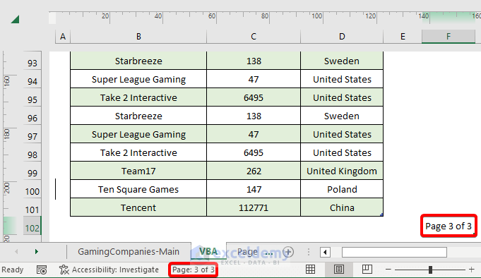
Thank you very much for reading our articles. You want to add the page number in the cell following the method Inserting Page Number in Excel Cell. You mentioned that every time you run the code and get “Page 1 of 9”, even in the last cell where it is supposed to show “Page 9 of 9”. Based on your complaint, we checked all the steps and run the VBA code again. We get an accurate result. See the image below.
I think you need to check the Status Bar at the bottom of the sheet, where the page number shows. We get the same result showing in the Status Bar after running the VBA code.
Hi HASNAIN AHMAD,
Thank you very much for following our article. You mentioned that even after changing the format of the Date_Time column, it did not work properly. To understand your problem, we follow the full process again and found everything is working properly. We suggest you read the steps again and apply them carefully. Hope you will get the desired result.
Dear PRATIK,
Thanks very much for reading our articles. You have mentioned that you have different lists in a single sheet. Here, we will show how to declare data validation in different cells with different lists in a single sheet.
Steps:
● Here, we have three different lists of mobile, laptop, and routers. Here, we will introduce different drop-down lists with multiple selections.
● Now, apply data validation as shown in the article already.
● We will choose Range B5:B11 at Cell G4, Range C5:C11 at Cell G5, and Range D5:D11 at Cell G6 for the data-validation source.
● Choose any item from the drop-down list of Cell G4.
● Similarly, choose items for Cell G5 and G6 from the drop-down list.
● Now, put the following VBA code in the VBA module. After that, save the VBA code.
Private Sub Worksheet_Change(ByVal Target As Range)
Dim Oldvalue As String
Dim Newvalue As String
On Error GoTo Exitsub
If Target.Column = 7 Then
If Target.SpecialCells(xlCellTypeAllValidation) Is Nothing Then
GoTo Exitsub
Else: If Target.Value = “” Then GoTo Exitsub Else
Application.EnableEvents = False
Newvalue = Target.Value
Application.Undo
Oldvalue = Target.Value
If Oldvalue = “” Then
Target.Value = Newvalue
Else
Target.Value = Oldvalue & “, ” & Newvalue
End If
End If
End If
Application.EnableEvents = True
Exitsub:
Application.EnableEvents = True
End Sub
● Now, choose multiple options from the drop-down list.
Here, we changed the Target.Address to Target.Column and put the column number. Also, need to mention the whole column will save the previous result.
Dear JEREMIAH,
Thanks for following our article. Here, you have mentioned that after an update you are not getting the default Zoom feature of Excel Online. But we are not facing such kind of problem. Also, one thing needs to add that, when we zoom any Excel sheet that will zoom in or out throughout the sheet, not in specific rows or cells. If we want to apply zoom in or out of a specific row or cell, we have to customize the length and width of that row or cell.
Are you still facing this problem?
Dear RENEE,
Thanks for following our articles. You mentioned a problem regarding the sheet name. Your sheet name will depend on the value of vcol variable. And one thing the sheets will split depending on the value of the 1st column which is the 1st column of the dataset. And, your provided code is not working due to some mistakes. You have made a mistake by setting the of vcol 7. Set the value of vcol as 1. Furthermore, use the below VBA that will solve your problem correctly.
Sub parse_data()
Dim lr As Long
Dim ws As Worksheet
Dim vcol, i As Integer
Dim icol As Long
Dim myarr As Variant
Dim title As String
Dim titlerow As Integer
‘This macro splits data into multiple worksheets based on the variables on a column found in Excel.
‘An InputBox asks you which columns you’d like to filter by, and it just creates these worksheets.
Application.ScreenUpdating = False
vcol = 1
Set ws = ActiveSheet
lr = ws.Cells(ws.Rows.Count, vcol).End(xlUp).Row
title = “A1”
titlerow = ws.Range(title).Cells(1).Row
icol = ws.Columns.Count
ws.Cells(1, icol) = “Unique”
For i = 2 To lr
On Error Resume Next
If ws.Cells(i, vcol) <> “” And Application.WorksheetFunction.Match(ws.Cells(i, vcol), ws.Columns(icol), 0) = 0 Then
ws.Cells(ws.Rows.Count, icol).End(xlUp).Offset(1) = ws.Cells(i, vcol)
End If
Next
myarr = Application.WorksheetFunction.Transpose(ws.Columns(icol).SpecialCells(xlCellTypeConstants))
ws.Columns(icol).Clear
For i = 2 To UBound(myarr)
ws.Range(title).AutoFilter field:=vcol, Criteria1:=myarr(i) & “”
If Not Evaluate(“=ISREF(‘” & myarr(i) & “‘!1)”) Then
Sheets.Add(after:=Worksheets(Worksheets.Count)).Name = myarr(i) & “”
Else
Sheets(myarr(i) & “”).Move after:=Worksheets(Worksheets.Count)
End If
ws.Range(“A” & titlerow & “:A” & lr).EntireRow.Copy Sheets(myarr(i) & “”).Range(“A1”)
‘Sheets(myarr(i) & “”).Columns.AutoFit
Next
ws.AutoFilterMode = False
ws.Activate
Application.ScreenUpdating = True
End Sub
Mr. Bhavnesh
Please read the following article and the 1st comment. Hopefully, you will get your answer.
Creation of a Mortgage Calculator with Taxes and Insurance in Excel
For further queries, please email us at [email protected].
Hi BHAVNESH,
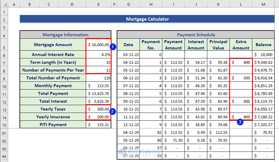
Thank you very much for reading our article. For different clients, you can create separate sheets using our Excel template. Yes, it is possible to change the interest rate. Also, that will change all the values accordingly. You can see in the below image, we changed the interest rate from 5% to 6.5%. Due to auto-update, all the values changed automatically.
You can also change other input values marked by 1. You can change the yearly insurance and taxes rate if changes. There is also the option to change the extra payment in Excel. You can use the IPMT function to calculate the interest part only. For penalty, please describe the situation or share your wordbook. After that, we try to solve that problem. You can mail us at [email protected].
Hello KO,
Thank you very much for your comment. The formula you mentioned in the comment is working smoothly from our side. If you share your workbook, we will be able to find out the solution to your problem. You can mail us at [email protected].
Dear RAZAN,
Thank you very much for reading our articles. Here, you mentioned that you do not want to get the answer in the form of Yes or No. You want to get the result in numbers. To solve your problem we formed a new formula based on the combination of the SUMPRODUCT, SUBSTITUTE, and LEN functions. Here is the formula:
=SUMPRODUCT((LEN($B$5:$B$19)-LEN(SUBSTITUTE($B$5:$B$19,$D5,"")))/LEN($D5))This formula will find out the specific word from the Range B5:B19 and return the sum in number.
If you want to get the number of a specific word from each cell you can follow this article.
Excel Formula to Count Specific Words in a Cell (3 Examples)
Hi MIRA,
It’s a great pleasure that you are watching our articles. You have a query regarding this article. You want to make an Excel sheet, where the dates of the Excel sheet will change according to the sheet name. Yes, you can do this. Read the below steps to get your solution.
Steps:
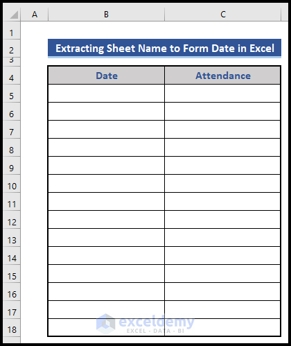
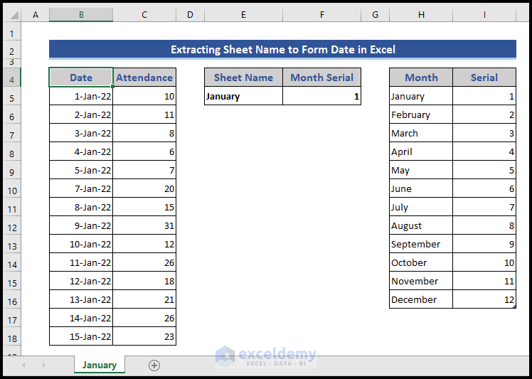
● First, take an Excel sheet with the Date and Attendance columns.
We will insert dates in the Date column based on the Sheet Name.
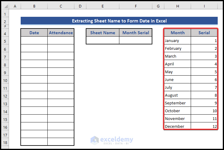
● Before that, we will form a table that consists of the month’s name and serial number.
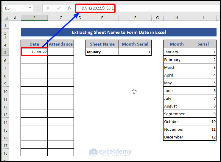
● Now, go to Cell E5 and put in the following formula.
=MID(CELL("filename",A1),FIND("]",CELL("filename",A1))+1,256)It will extract the name of the Sheet which is a month name.
Formula Explanation:
● CELL(“filename”,A1)
This finds the location of the Excel file with the Sheet name.
Result:
D:\Alok\[Excel-Sheet-Name-From-Cell-Value.xlsx]January
● FIND(“]”,CELL(“filename”,A1))
This will find out the location of the symbol mentioned in the formula from the location.
Result: 47
● FIND(“]”,CELL(“filename”,A1))+1
Add 1 with the previous result.
Result: 48
● MID(CELL(“filename”,A1),FIND(“]”,CELL(“filename”,A1))+1,256)
Separate the sheet name from the location.
Result: January
● After that, put the following formula on Cell F5.
=INDEX(Month,MATCH(E5,Month[Month],0),2)
This returns the serial number of the month comparing the values of the table.
● Now, use the DATE function on Cell B5.
=DATE(2022,$F$5,1)
● Fill up the Date and Attendance columns.
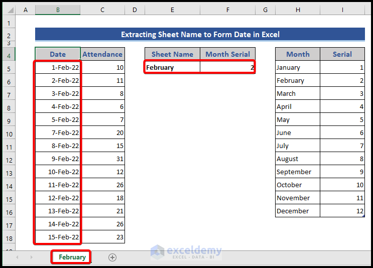
● Now, change the sheet name from January to February and look at the changes that take place in the Date column.
Download File:
Solution.xlsx
Regards.
– Alok Paul
Author at ExcelDemy
Hi JORGE,
It’s a bit difficult to answer this, not seeing your spreadsheet. Can you please send a sample to [email protected]?
Prior to that, check the following Excel file. We have added a 12-month example for you. Let us know if this helps.
Download Link:
Solution.xlsx
Note:
You must have data of 2021 and 2022 for forecasting 2023.
Hello, JITENDRA!
Hope you are doing well. You have a query to get the product name and min & max sell price monthly basis. We have to use the following formulas for that.
For Max values:
=MAXIFS($E$5:$E$17,$D$5:$D$17,$G$4)
For Min values:
=MINIFS($E$5:$E$17,$D$5:$D$17,$G$4)
For Product Name:
=INDEX($B$5:$E$17,MATCH($J$6,$E$5:$E$17,0),1)
We just need to change the month name of Cell G4. Hope you will get your desired solution. Regards
-Alok Paul
Author at ExcelDemy
Hi JUAN MARTIN OPACAK,
Thanks for reading our articles. We have found a solution to fulfill your requirement. You need to insert the following macros with the existing VBA code.
Worksheets(ActiveSheet.Index + 1).SelectActiveSheet.Name = (Worksheets(2).Range("A1").Value) & " " & ActiveSheet.NameHere, Worksheets(2).Range(“A1”).Value defines we want to insert the text of Cell A1 of Worksheet 2 with the current sheet name.
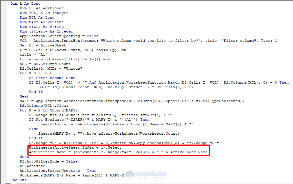
Have a look at the image below, where to insert the mentioned VBA code.
Hi NAYAZ,
Thanks for following our article. We have checked the article again and found no errors. Please go through the whole article again and create the template. Or you can do this easily by downloading the given template.
Keep in mind that if you want to import stock prices from any other website, then it will not work. You should use “^NSEI” in the ticker box.
Let us know if your problem is fixed.
Regards.
-Alok Paul
Author at ExcelDemy
Hello, DANIEL.
Thanks for reading our articles.
Look at the below link. Hopefully, you will get your solution.
https://www.exceldemy.com/extract-data-from-one-sheet-to-another-in-excel-using-vba/
For example, you can use the following code:
Sub Extract_Data()Selection.CopySheets("Dataset2").ActivateRange("F4").SelectActiveSheet.PasteApplication.CutCopyMode = FalseEnd SubEnter your sheet name instead of Dataset2 in the 3rd line. Change the cell range in the 4th line. Hope you will get desired output. If your problem is yet solved, then let us know.
Regards.
-Alok Paul
Author at ExcelDemy
Hello, CL.
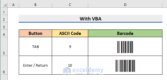
Of course, it’s possible to solve your mentioned problem!
You will need to get the ASCII code of the respective keys. Now, open a new Excel file and follow all the steps written in this article, i.e. downloading Barcode fonts 128, installing them, creating a UDF, and the next steps. Now insert the ASCII codes of the respective keys and you will get your desired Barcode. See what we have got.
So, what you need to do yourself, just finding the ASCII codes! What else to do are already mentioned in this article.
Note: You may need to open a new file because as per the new update of Excel, a VBA code will be disabled in a downloaded xlsm file. Or you can solve the problem following this way.
Hi DAVID,
Thank you very much for your appreciation. Follow our website ExcelDemy for other problems, and hope you will always get the best solutions.
Hello JEFF WHALE,
Thank you very much for following our articles.
You mentioned that your sample code is not working properly. We attached a VBA code that will help you to solve this problem. You need to choose a cell from the dataset that contains an ISBN number when running the code. One thing adding that change the location of Chrome according to your computer.
And you are getting this 404 error because without any ISBN number, this isbnsearcher.com/books link will show an error by default.
Sub OpenstrHyperlinkInChrome()Dim strChromeLocation As StringDim strURL As StringDim strISBN As StringstrISBN = Application.InputBox("Please Select Desired Cell", Type:=8)strURL = "https://www.isbnsearcher.com/books/" & strISBNstrChromeLocation = """C:\Program Files\Google\Chrome\Application\chrome.exe"""Shell (strChromeLocation & "-url " & strURL)End SubHi BARNEY! Hope you are doing well. Thanks for your nice compliments. We are happy to know that the readers find our articles useful.
However, the problem you are facing is not quite clear from what you have told us. Are you trying to sum up entries that meet specific criteria? In that case, you have to use the SUMIF function if you have to meet just a single criterion. If you have multiple criteria, then you have to use the SUMIFS function. There are more articles in our blog related to these functions. To explore them, scroll down and click on the function tag names.
If this is not what you are looking for, please let us know more details. You can send me the problem with a sample file at [email protected] or at [email protected].
Best wishes. Keep staying with us.
-Alok Paul
ExcelDemy Team
Hi KATIE WILDER,
You probably have missed this part. The solution to your problem is already given in the article.
Click the below link and will get the solution.
https://www.exceldemy.com/make-excel-read-only-with-password/#Disable_Excel_Read-only-recommended_Option
If I am not wrong, this is what you are searching for. As far as we know, you cannot undo protection to a password-protected file, but save a copy of it without password protection. If this is not your case, please let us know a bit more details.
Thanks for being with us.
Hi JEFF! Thanks for your nice compliment. To remove the InputBox and make the code always select Column 1, just remove the InputBox command and variable VCL. After that, replace the VCL with 1.
You can directly use the following code:
Sub Split_Data()Dim L As LongDim DS As WorksheetDim XCL As LongDim MARY As VariantDim title As StringDim titlerow As IntegerApplication.ScreenUpdating = FalseSet DS = ActiveSheetL = DS.Cells(DS.Rows.Count, 1).End(xlUp).Rowtitle = "A1"titlerow = DS.Range(title).Cells(1).RowXCL = DS.Columns.CountDS.Cells(3, XCL) = "Unique"For X = 2 To LOn Error Resume NextIf DS.Cells(X, 1) <> "" And Application.WorksheetFunction.Match(DS.Cells(X, 1), DS.Columns(XCL), 0) = 0 ThenDS.Cells(DS.Rows.Count, XCL).End(xlUp).Offset(1) = DS.Cells(X, 1)End IfNextMARY = Application.WorksheetFunction.Transpose(DS.Columns(XCL).SpecialCells(xlCellTypeConstants))DS.Columns(XCL).ClearFor X = 2 To UBound(MARY)DS.Range(title).AutoFilter field:=1, Criteria1:=MARY(X) & ""If Not Evaluate("=ISREF('" & MARY(X) & "'!A1)") ThenSheets.Add(after:=Worksheets(Worksheets.Count)).Name = MARY(X) & ""ElseSheets(MARY(X) & "").Move after:=Worksheets(Worksheets.Count)End IfDS.Range("A" & titlerow & ":A" & L).EntireRow.Copy Sheets(MARY(X) & "").Range("A4")NextDS.AutoFilterMode = FalseDS.ActivateApplication.ScreenUpdating = TrueEnd SubYou are most welcome, MANUEL!
We provide the best and easy solutions to Excel-related problems. You are invited to visit our blog for more such articles.
If the last two rows contain the same data, then it fails to delete both rows. Otherwise, it works.