In this article, we describe how to split data into multiple Excel worksheets using VBA & Macros.
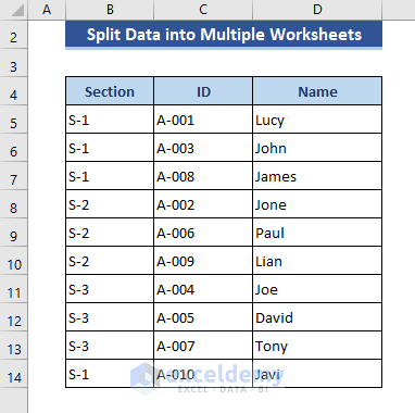
In our data set, we have data comprising student names, IDs, and sections.
Step 1 – Create a New Macro in VBA Module
We will split data into different worksheets based on the column.
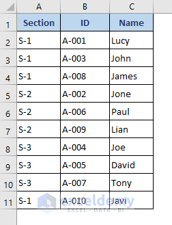
To perform this method, we always need to start data from Cell A1.
- Copy the data and paste it into another sheet at Cell A1.
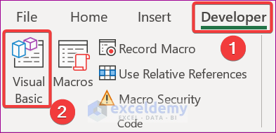
- Choose the Developer tab.
- Click on Visual Basic from the Code group.
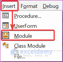
- Click on Insert → Module.
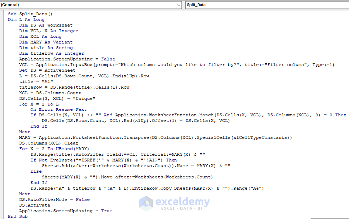
- Enter the below code in the Module box:
Sub Split_Data()
Dim L As Long
    Dim DS As Worksheet
    Dim VCL, X As Integer
    Dim XCL As Long
    Dim MARY As Variant
    Dim title As String
    Dim titlerow As Integer
    Application.ScreenUpdating = False
    VCL = Application.InputBox(prompt:="Which column would you like to filter by?", title:="Filter column", Type:=1)
    Set DS = ActiveSheet
    L = DS.Cells(DS.Rows.Count, VCL).End(xlUp).Row
    title = "A1"
    titlerow = DS.Range(title).Cells(1).Row
    XCL = DS.Columns.Count
    DS.Cells(3, XCL) = "Unique"
    For X = 2 To L
        On Error Resume Next
        If DS.Cells(X, VCL) <> "" And Application.WorksheetFunction.Match(DS.Cells(X, VCL), DS.Columns(XCL), 0) = 0 Then
            DS.Cells(DS.Rows.Count, XCL).End(xlUp).Offset(1) = DS.Cells(X, VCL)
        End If
    Next
    MARY = Application.WorksheetFunction.Transpose(DS.Columns(XCL).SpecialCells(xlCellTypeConstants))
    DS.Columns(XCL).Clear
    For X = 2 To UBound(MARY)
        DS.Range(title).AutoFilter field:=VCL, Criteria1:=MARY(X) & ""
        If Not Evaluate("=ISREF('" & MARY(X) & "'!A1)") Then
            Sheets.Add(after:=Worksheets(Worksheets.Count)).Name = MARY(X) & ""
        Else
            Sheets(MARY(X) & "").Move after:=Worksheets(Worksheets.Count)
        End If
        DS.Range("A" & titlerow & ":A" & L).EntireRow.Copy Sheets(MARY(X) & "").Range("A4")
    Next
    DS.AutoFilterMode = False
    DS.Activate
    Application.ScreenUpdating = True
End Sub
Step 2 – Save the File in XLSM Format and Run the Macro
- Press F5 to run the code.
A dialog box will appear to input a number.
- Put 1 here, as we want to split data based on Column 1.
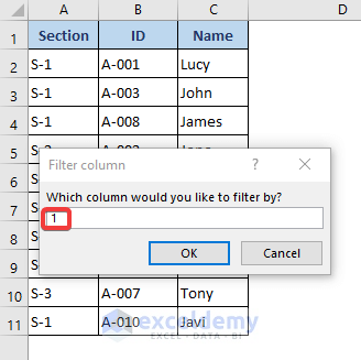
- Click OK.
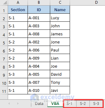
We can see that the data are in the S-1, S-2, and S-3 sheets now.
- Open the S-1 sheet.
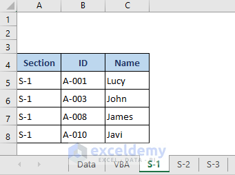
All data regarding the S-1 section is here. Data started from Cell A4 because we set this condition in the VBA code.
Code Explanation:
Dim L As Long
Dim DS As Worksheet
Dim VCL, X As Integer
Dim XCL As Long
Dim MARY As Variant
Dim title As String
Dim titlerow As Integer
>> Declares different variables.
Application.ScreenUpdating = False>> Defines whether the screen will update or not. Here, False stops updating. Screen update is turned off to speed up the macro.
VCL = Application.InputBox(prompt:="Which column would you like to filter by?", title:="Filter column", Type:=1)>>Introduces an input box, into which we will input the column number.
Set DS = ActiveSheet>> Fixes the active sheet as the value of the DS variable.
L = DS.Cells(DS.Rows.Count, VCL).End(xlUp).Row>> DS.Cells(DS.Rows.Count, VCL) defines that our reference is a cell of column VCL located at the last row of the DS sheet. End(xlUp) chooses the last or first row in the upward direction.
titlerow = DS.Range(title).Cells(1).Row>> Indicates the first row as the title.
XCL = DS.Columns.Count>> Counts the number of columns into the XCL variable.
DS.Cells(3, XCL) = "Unique">> Names the range as “Unique”
For X = 2 To L>> Uses For loop to set the value of X from 2 to L
On Error Resume Next>> If any error is found, resumes the operation and goes to the Next section.
If DS.Cells(X, VCL) <> "" And Application.WorksheetFunction.Match(DS.Cells(X, VCL), DS.Columns(XCL), 0) = 0 Then
DS.Cells(DS.Rows.Count, XCL).End(xlUp).Offset(1) = DS.Cells(X, VCL)
End If
>> Applies a condition using the worksheet Match function.
MARY = Application.WorksheetFunction.Transpose(DS.Columns(XCL).SpecialCells(xlCellTypeConstants))>> Uses the worksheet Transpose function on the line.
DS.Columns(XCL).Clear>> Clears the contents of the Column marked by the XCL variable.
For X = 2 To UBound(MARY)>> Applies a For loop, with the value of the X set from 2 to the upper limit of the array MARY variable.
DS.Range(title).AutoFilter field:=VCL, Criteria1:=MARY(X) & "">> Sets the VCL variable as the range of AutoFilter.
If Not Evaluate("=ISREF('" & MARY(X) & "'!A1)") Then
Sheets.Add(after:=Worksheets(Worksheets.Count)).Name = MARY(X) & ""
Else
Sheets(MARY(X) & "").Move after:=Worksheets(Worksheets.Count)
End If
>> Sets another IF condition.
DS.Range("A" & titlerow & ":A" & L).EntireRow.Copy Sheets(MARY(X) & "").Range("A4")>> Copies the data of the whole row.
DS.AutoFilterMode = False>> Removes the arrow symbol of the filter drop-down.
DS.Activate>> Activates the worksheet of the DS variable.
Application.ScreenUpdating = True>> Enables screen updating by setting the value True.
Read More: Excel Macro to Split Data into Multiple Files
Download Practice Workbook
Related Articles
- How to Split Data into Equal Groups in Excel
- Excel Split Data into Columns by Comma
- How to Split Comma Separated Values into Rows or Columns in Excel
- How to Split Data into Multiple Columns in Excel
- How to Split Data from One Cell into Multiple Rows in Excel


I think I would need more information on how the code actually works in order to get it to work for me. I was trying it on my own data, but I keep getting an overflow error on the line: For X = 2 To L
I swear I got it to work once, but then the excel file broke, and I lost all the progress. Just having a block of code isn’t super helpful if there aren’t notations explaining what the parts do so we know how to adjust it if need be.
We are extremely sorry Hannah W. to know that you have faced this difficulty in applying our provided code! We have added the code explanation. Is your problem solved? Please let us know.
With regards
-ExcelDemy team
Not worked
The code is perfectly working from our end, Goel! Can you please send your problem to this email: [email protected]?
Works great, thank you! How do you remove the InputBox and make it always select Column 1?
Hi JEFF! Thanks for your nice compliment. To remove the InputBox and make the code always select Column 1, just remove the InputBox command and variable VCL. After that, replace the VCL with 1.
You can directly use the following code:
Sub Split_Data()Dim L As LongDim DS As WorksheetDim XCL As LongDim MARY As VariantDim title As StringDim titlerow As IntegerApplication.ScreenUpdating = FalseSet DS = ActiveSheetL = DS.Cells(DS.Rows.Count, 1).End(xlUp).Rowtitle = "A1"titlerow = DS.Range(title).Cells(1).RowXCL = DS.Columns.CountDS.Cells(3, XCL) = "Unique"For X = 2 To LOn Error Resume NextIf DS.Cells(X, 1) <> "" And Application.WorksheetFunction.Match(DS.Cells(X, 1), DS.Columns(XCL), 0) = 0 ThenDS.Cells(DS.Rows.Count, XCL).End(xlUp).Offset(1) = DS.Cells(X, 1)End IfNextMARY = Application.WorksheetFunction.Transpose(DS.Columns(XCL).SpecialCells(xlCellTypeConstants))DS.Columns(XCL).ClearFor X = 2 To UBound(MARY)DS.Range(title).AutoFilter field:=1, Criteria1:=MARY(X) & ""If Not Evaluate("=ISREF('" & MARY(X) & "'!A1)") ThenSheets.Add(after:=Worksheets(Worksheets.Count)).Name = MARY(X) & ""ElseSheets(MARY(X) & "").Move after:=Worksheets(Worksheets.Count)End IfDS.Range("A" & titlerow & ":A" & L).EntireRow.Copy Sheets(MARY(X) & "").Range("A4")NextDS.AutoFilterMode = FalseDS.ActivateApplication.ScreenUpdating = TrueEnd SubI’m getting the same error. I’d love to know what I’m doing wrong.
Dear HEATHER, I guess you are facing the same problem as HANNAH. But we have rechecked the code, and applied it again, but have found no issue.
Can you please send us your problem with specific details? Here is our address: [email protected]
We have added the code explanation. Have a look at it and let us know if it can do any help regarding your problem. But the best will be to send your problem in detail with your Excel file. Thanks and regards.
-ExcelDemy Team
Works great.
However, would it be possible to change the names of the newly created sheets?
Using your example, the generated sheets were named “S-1”, “S-2”, “S-3”.
How would you modify the code to set them to “Section S-1”, “Section S-2”, “Section S-3”? (where ‘Section’ is a text value copied from cell A1 – or any other)
Thank you!
Hi JUAN MARTIN OPACAK,
Thanks for reading our articles. We have found a solution to fulfill your requirement. You need to insert the following macros with the existing VBA code.
Worksheets(ActiveSheet.Index + 1).SelectActiveSheet.Name = (Worksheets(2).Range("A1").Value) & " " & ActiveSheet.NameHere, Worksheets(2).Range(“A1”).Value defines we want to insert the text of Cell A1 of Worksheet 2 with the current sheet name.
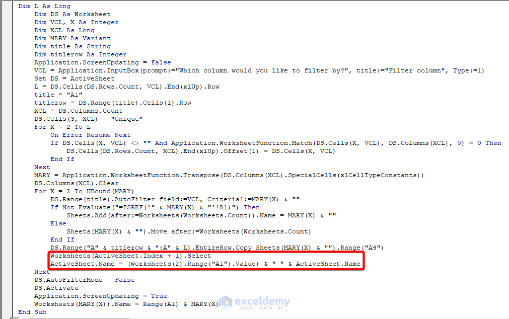
Have a look at the image below, where to insert the mentioned VBA code.
I have been using a similar macro but am now noticing that I am getting additional sheets added with names like Sheet 15, Sheet 30. Any idea why? Here is the macro I’ve used.
Sub parse_data()
Dim lr As Long
Dim ws As Worksheet
Dim vcol, i As Integer
Dim icol As Long
Dim myarr As Variant
Dim title As String
Dim titlerow As Integer
‘This macro splits data into multiple worksheets based on the variables on a column found in Excel.
‘An InputBox asks you which columns you’d like to filter by, and it just creates these worksheets.
Application.ScreenUpdating = False
vcol = 7
Set ws = ActiveSheet
lr = ws.Cells(ws.Rows.Count, vcol).End(xlUp).Row
title = “A1”
titlerow = ws.Range(title).Cells(1).Row
icol = ws.Columns.Count
ws.Cells(1, icol) = “Unique”
For i = 2 To lr
On Error Resume Next
If ws.Cells(i, vcol) “” And Application.WorksheetFunction.Match(ws.Cells(i, vcol), ws.Columns(icol), 0) = 0 Then
ws.Cells(ws.Rows.Count, icol).End(xlUp).Offset(1) = ws.Cells(i, vcol)
End If
Next
myarr = Application.WorksheetFunction.Transpose(ws.Columns(icol).SpecialCells(xlCellTypeConstants))
ws.Columns(icol).Clear
For i = 2 To UBound(myarr)
ws.Range(title).AutoFilter field:=vcol, Criteria1:=myarr(i) & “”
If Not Evaluate(“=ISREF(‘” & myarr(i) & “‘!A1)”) Then
Sheets.Add(after:=Worksheets(Worksheets.Count)).Name = myarr(i) & “”
Else
Sheets(myarr(i) & “”).Move after:=Worksheets(Worksheets.Count)
End If
ws.Range(“A” & titlerow & “:A” & lr).EntireRow.Copy Sheets(myarr(i) & “”).Range(“A1”)
‘Sheets(myarr(i) & “”).Columns.AutoFit
Next
ws.AutoFilterMode = False
ws.Activate
Application.ScreenUpdating = True
End Sub
Dear RENEE,
Thanks for following our articles. You mentioned a problem regarding the sheet name. Your sheet name will depend on the value of vcol variable. And one thing the sheets will split depending on the value of the 1st column which is the 1st column of the dataset. And, your provided code is not working due to some mistakes. You have made a mistake by setting the of vcol 7. Set the value of vcol as 1. Furthermore, use the below VBA that will solve your problem correctly.
Sub parse_data()
Dim lr As Long
Dim ws As Worksheet
Dim vcol, i As Integer
Dim icol As Long
Dim myarr As Variant
Dim title As String
Dim titlerow As Integer
‘This macro splits data into multiple worksheets based on the variables on a column found in Excel.
‘An InputBox asks you which columns you’d like to filter by, and it just creates these worksheets.
Application.ScreenUpdating = False
vcol = 1
Set ws = ActiveSheet
lr = ws.Cells(ws.Rows.Count, vcol).End(xlUp).Row
title = “A1”
titlerow = ws.Range(title).Cells(1).Row
icol = ws.Columns.Count
ws.Cells(1, icol) = “Unique”
For i = 2 To lr
On Error Resume Next
If ws.Cells(i, vcol) <> “” And Application.WorksheetFunction.Match(ws.Cells(i, vcol), ws.Columns(icol), 0) = 0 Then
ws.Cells(ws.Rows.Count, icol).End(xlUp).Offset(1) = ws.Cells(i, vcol)
End If
Next
myarr = Application.WorksheetFunction.Transpose(ws.Columns(icol).SpecialCells(xlCellTypeConstants))
ws.Columns(icol).Clear
For i = 2 To UBound(myarr)
ws.Range(title).AutoFilter field:=vcol, Criteria1:=myarr(i) & “”
If Not Evaluate(“=ISREF(‘” & myarr(i) & “‘!1)”) Then
Sheets.Add(after:=Worksheets(Worksheets.Count)).Name = myarr(i) & “”
Else
Sheets(myarr(i) & “”).Move after:=Worksheets(Worksheets.Count)
End If
ws.Range(“A” & titlerow & “:A” & lr).EntireRow.Copy Sheets(myarr(i) & “”).Range(“A1”)
‘Sheets(myarr(i) & “”).Columns.AutoFit
Next
ws.AutoFilterMode = False
ws.Activate
Application.ScreenUpdating = True
End Sub
This macro is great, thank you for sharing it!
It works very well to split my data, however I only need to copy the lines from column A to J, not the entire row. I am very new to VBA/macros and am having trouble figuring out how to do this myself. Could you please help?
Hello CASSIE,
Greetings. Use Excel VBA to quickly complete your task. In Excel VBA, you can use the following code to only copy the cells in columns A through J (inclusive) rather than the entire row:
The End(xlUp) method, which locates the final non-empty cell in the column, is used in this code to obtain the last row in column A first. Then, using the Range object and Copy method, it copies the data from columns A to J.
This code can be changed if you want to perform additional operations on the copied data or paste it in a different place.
Thank you really much!
That’s right what I needed. With some small adjustements, I can now split my “database” by filtering on a specific column.
Hello Joel,
You are most welcome.
Regards
ExcelDemy
This code is great! Thank you so much!
How can I get it to just copy the rows of data without the 2 header rows duplicated on each worksheet?
Hi RED,
Thanks for reading our articles. Hope you are doing well.
You want to copy the rows of data without the header row duplicated on each worksheet.
There may be two situations:
Case 1: The header row will not exist in any of the split worksheets.
Case 2: The header row will exist on the first split worksheet.
For Case 1: Change the 13th line of the current VBA code from title = “A1” to title = “A2”. After making this adjustment and running the VBA, the header row will not be visible in the split worksheets.
For case 2: We added a variable named isFirstSheet to distinguish the first split sheet, displaying the header row, and excluding it from subsequent sheets. Employ the updated VBA code provided below:
We have marked the modified section of the VBA code in the above image.
Best Regards,
Alok
Team ExcelDemy
Hi, Thanks! This works perfectly. Can you tell me how do I use the same parameters and split into multiple files instead of workbooks?
Hello Vini,
Updated the code spilt data into multiple Excel file.
Regards
ExcelDemy
Hi, I used the VBA but the tabs had extra rows on the top and did not keep the spacing column formatting or top row froze or kept the filters on. Still, this is super helpful 🙂 Many thanks!
Hello Susan,
You are most welcome and thanks a lot for your feedback. Basic VBA usually focuses on splitting the data, so things like extra blank rows, column spacing, frozen top rows, and filters don’t always carry over by default.
The good news is that all of these can be preserved with a few small additions to the code (for example, copying row heights, column widths, applying FreezePanes, and re-enabling filters after the split). If you’d like, you can share which formatting is most important for your case, and the VBA can be adjusted accordingly.
Really glad to hear the article was still helpful. Many thanks for taking the time to comment!
Regards,
ExcelDemy