Latest Posts From Akib Bin Rashid

Excel is the most widely used tool for dealing with massive datasets. We can perform myriads of tasks of multiple dimensions in Excel. This article will show ...

Excel is the most widely used tool for dealing with massive datasets. We can perform tasks of multiple dimensions in Excel. I will show you how to create a ...

Excel is the most widely used tool for dealing with massive datasets. We can perform myriads of tasks of multiple dimensions in Excel. I will show you how to ...

Introduction to the Cumulative Probability The cumulative probability is the likelihood that the value of a random variable is within a specific range. ...

Excel is the most widely used tool for dealing with massive datasets. We can perform myriads of tasks of multiple dimensions in Excel. In this article, I will ...

Introduction to the 360 Interest Calculation System Actual/360, also known as the 365/360 rule, is the most frequently used method by banks to calculate ...
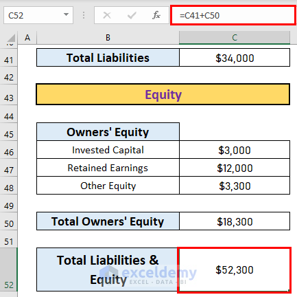
In this article, we will explain how to create a balance sheet format for a trading company in Excel. Introduction to Balance Sheet Projected balance ...
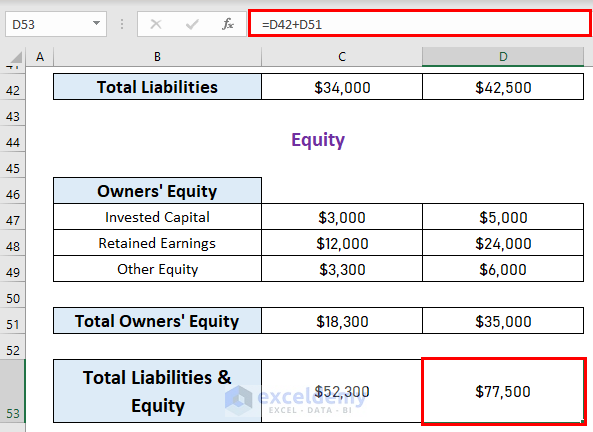
Method 1 - Create Format Outline The balance sheet should start with a heading followed by the company’s name and the date it is being created. This is what ...

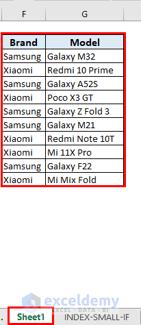
Here is the dataset for today’s article. There are some orders with due dates and amounts. We will calculate the Aging of Accounts Receivable using this ...

Excel is the most widely used tool for dealing with massive datasets. We can perform myriads of tasks of multiple dimensions in Excel. In this article, I will ...
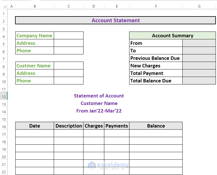
Watch Video – Create an Account Statement in Excel Step 1: Prepare an Appropriate Outline The first step is to create an ...

This is the sample dataset. Step 1 - Create a New Module in Visual Basic Window Select Developer. Choose Visual Basic. In the VBA ...

This is the sample dataset: Step 1 - Plot a Chart using the Insert Tab Go to the Insert tab. Select Scatter. Choose a type of scatter ...

Method 1 -Using Multiplication to Convert Hours and Minutes to Minutes in Excel The relationship between time units is, 1 Day = 24 Hours = 24*60 or 1440 ...

The Weibull Distribution is a continuous probability distribution that is used to analyze life data, model failure times, and assess the reliability of access ...
- « Previous Page
- 1
- 2
- 3
- 4
- 5
- …
- 9
- Next Page »
See Our Reviews at


Hi HAZEL,
I am assuming that you want to transfer Gender and Language from one column to another without changing the row position.
In that case, you can insert a new column to the left of the Gender and Language column.
To do so,
● Select the Gender column.
● Then, right-click your mouse to bring the context menu.
● After that, select Insert.
● Excel will add a new column and transfer the Gender and Language column.\
There is another solution to this problem. You can use the OFFSET function. The advantage of this function is that you can transfer any portion of the columns to anywhere in the Excel sheet.
Suppose, I want to transfer B8:C10 to E8:F10. To do so,
● Go to E8 and write down the following formula
=OFFSET(B4,4,0,3,2)
● Then, press ENTER. Excel will move the cells.
● If you use earlier versions of Excel, you have to select E8:F10, then write down the formula and finally press CTRL+SHIFT+ENTER, since the OFFSET function is an array function.
And lastly, you can copy the cells and paste them to transfer columns.
I hope it helps. If it does not satisfy you, please let us know.
Thank you. Have a great day.
Hi LILIA,
 \
\
I hope you are doing well.
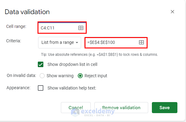
Please use the conditions as per the image and see if it works.
The range $E$4:$E$100 will allow you to have a list of 97 items. So, this can be used as a dynamic drop-down
Thank you.
Hi KALI,
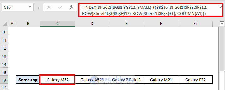
Normally when we write down a formula that has references from multiple sheets, the sheet name appears first. That’s why “Data range” appears. You can check the final image of step 3 to get the final formula.
‘Data range’!’Data range’!C5:G19 is corrected now. Thank you for your observation.
‘Data range’!$B$5:$B$10 refers to the range B5:B10. The selected range starts from the 5th row to the 10th row of column B.
Thanks again. Have a good day.
Hi DAVID,
I hope you are doing well.
In Excel, you cannot do so as far as I know. However, you can make the fill color same as the background color to technically avoid printing the row.
And you can also hide specific rows and columns to not print them.
Thank you. Have a good day.
Hi HAIVH
Let me first clear up your confusion.
• Normally, when you pay a certain amount, you have cash outflow. Hence the amount you pay becomes negative.
• On the other hand, when you receive a certain amount, you have cash inflow. Hence the amount you get becomes positive.
Coming to your problem,
• PMT function is used to calculate the monthly payment for a loan. This problem is not a case of loan payment. So, I think the PMT function is not suitable to be used here.
Hello STEEN and DAV,
I have checked the methods on several laptops. They are working well here.
For your convenience, I have added a new Excel file with the VBA code.
Please download it and check if the methods are working.
Thank you. Have a good day.
Hi DOMINIC,
Yes, it’s possible to join non-consecutive cells using the TEXTJOIN Function in Excel.
Let me show you how you can do it.
Let’s assume this is your dataset.
Then, in A8, apply the following formula
=TEXTJOIN(",",TRUE,A4:A6,A1)The delimiter is a comma (,)
TRUE indicates that you are going to ignore empty values.
Then, press ENTER to get the output.
I hope it helps.
Have a good day.
Hi SANKARSHAN
Generally, you can set one CRITERIA when you apply only COUNTIF Function.
However, if you use a formula that has multiple functions, you can set multiple criteria.
Let me show you an example.
● Suppose you have a set of fruits. You want to count the instances when the fruit is either Mango or Apple.
● Go to D5 and write down the following formula
=COUNTIF(B4:B15,B4)+COUNTIF(B4:B15,B5)Here, Excel will count the instances when the criteria is Mango or Apple from the same range B4:B15.
● Now, press ENTER to get the output.
I hope it helps.
You can also check the following articles to internalize the concept.
● COUNTIF with Multiple Criteria in Different Columns in Excel
● COUNTIFS with Multiple Criteria (5 Easy Methods)
Thank you.
Hi Casey,
You may not get the desired output if you download the excel file attached to this article and perform operations.
1. You must download the barcode font. The link is in the 1st step of this article
2. Also, code 128 has 106 distinct characters. Πis not available in code 128.
Maybe these are the 2 issues that need to be resolved.
However, if these don’t satisfy you, please let us know.
Have a great day!
Hi Marko
I hope you are doing well.
After going through your problem, I will give you 2 possible solutions.
Solution 1:
This will require you to insert the number after “WA11” within parentheses.
● Add the parentheses.
● Then, write down the following formula in B2.
=MID(A1,SEARCH("(",A1)+1, SEARCH(")",A1)-SEARCH("(",A1)-1)+0● Then, press ENTER. Excel will extract the number inside the parentheses.
● Then, AutoFill up to B3.
● Finally, add the numbers.
Solution 2:
● This will require you to have a helping column with the numbers with “WA11”. But this is a bit tedious if you have a lot of data.
● Now, add the numbers.
Hope this helps. Thank you.
Hi David
As far as I understand the case, you want to apply a filter to a row but keep the numbers in the cell permanent.
Unfortunately, when Excel executes a filter, it hides the entire row. If any cell contains numbers, excel will hide them too. However, as this article explains, you can maintain the serial when applying a filter.
In case I have misunderstood your requirement, please mail us the excel file at [email protected] and explain the problem a bit more.
Thank you.
Hi G0DWIN,
Thank you for your kind words!
Hi KRISB,
I hope you are doing well.
If you copy the table and paste it somewhere else, then Excel will not adjust cell references according to the move.
The formula should work fine if you cut the table and paste it into another sheet.
For instance, I have cut the table and pasted it into “sheet1”. Then Excel automatically modifies the formula. See the image for better clarification.
The table was shifted in “sheet1”
Hi NGÂN,
The solution you want will require a combination of some functions like TODAY, COUNTIF, VLOOKUP, etc. Here is a post on our website that will help you.
https://www.exceldemy.com/stock-ageing-analysis-formula-in-excel/
We have several posts related to this topic too.
https://www.exceldemy.com/make-inventory-aging-report-in-excel/
https://www.exceldemy.com/excel-ageing-formula-for-30-60-90-days/
https://www.exceldemy.com/aging-of-accounts-receivable-in-excel/
I hope these articles will help get your job done. If not, please remember that we are just a text away!!
Thank you. Have a good day.
Thank you for your kind words.
Have a good day!!
Dear Tiago
It’s good to know that you have finished your work successfully. No, I have not tried the MLE method for Weibull Distribution yet.
Thank you. Have a good day!
Dear Tiago
To implement suspension data in a Weibull Distribution, follow these steps:
•Collect completed failure data and suspended data.
•Estimate Weibull distribution parameters (shape and scale) using standard methods for completed data.
•Determine the truncation point for suspended data.
•Modify the Weibull PDF and CDF formulas to account for truncation.
•Estimate parameters for suspended data using methods that consider truncation.
•Evaluate the model’s fit using techniques like Q-Q plots or statistical tests.
Thank you.
Hello MAX
Thank you for your comment. I have examined the entire workbook properly. As per my understanding, the sheet works fine.
The “Monthly” option in Extra Payment Frequency will be available if you select the “Monthly” option in the Regular Payment Frequency field. Actually, the options in Extra Payment Frequency are dependent on the Regular Payment Frequency field.
Coming to the 2nd issue, the summary table updates properly on my device. In your case, could you please check the version of Excel you are operating? This sheet has some advanced functions that may not work in all Excel versions.
Please let us know if you are satisfied with this answer. If not, please feel free to ask us. You can even send your dataset to the following address: [email protected]
Thanks again. Have a good day!
Hi A
We haven’t shown step-by-step solutions because the underlying objective of this article is to help our users internalize these problems to the core. We strongly believe that this will be possible only if we give a generic guideline and let our users practice more.
Coming to your VLOOKUP issue, the formula you should use is =VLOOKUP(E5,’Reference Table’!$B$5:$C$11,2,0)
Please double-check that you have the cell references correct.
You can check the following articles
for VLOOKUP: https://www.exceldemy.com/excel-vlookup-function/
for referencing: https://www.exceldemy.com/difference-between-absolute-and-relative-reference-in-excel/
I think these two articles, along with the workbook attached to this article will solve your problem.
However, if these resources do not solve your problem, then please send us your workbook at [email protected]
Thank you for your patience.
Hi Mohammed
Thank you for your appreciation. If you want to incorporate ERC in your final balance, I think your method is a nice one.
I would, however, suggest one thing. Keep the ERC in column I and calculate the final balance in column J.
Hi Tom
Thank you for your query. The arrow (^) is called the caret symbol or circumflex symbol.
For a U.S. keyboard, hold down the Shift button and press the number key 6 at the top of the keyboard ( Shift + 6 ) to get a caret symbol.
Thank you
Hi Jack
Thank you for your query.
It would be very kind of you if explain your problem in detail. Perhaps, you can send us your problem at [email protected] to get better assistance.
From your query, it seems like you want to calculate in Excel using the RATE function and insert a certain fee as a percentage in the function.
The RATE function returns the interest rate per period of an annuity. The syntax of the RATE function is as follows.
RATE(nper, pmt, pv, [fv], [type], [guess])
Where,
● Nper: Required. The total number of payment periods in an annuity.
● Pmt: Required. The payment made each period and cannot change over the life of the annuity. Typically, pmt includes principal and interest but no other fees or taxes. If pmt is omitted, you must include the fv argument.
● Pv: Required. The present value — the total amount that a series of future payments is worth now.
● Fv: Optional. The future value, or a cash balance you want to attain after the last payment is made. If fv is omitted, it is assumed to be 0 (the future value of a loan, for example, is 0). If fv is omitted, you must include the pmt argument.
● Type: Optional. The number 0 or 1 and indicates when payments are due.
● Guess: Optional.
As you can see, you cannot directly incorporate any fee as a percentage in the RATE function. However, you can indirectly use a percentage in a formula that has the RATE function.
I am going to discuss 2 such examples.
Example 1:
Let’s assume that you have borrowed $8000 for 4 years. The monthly payment is $200. Now, if you use the RATE function here, you will get a 9.24% annual loan rate. But in practice, you may need to adjust your loan. So in that case, you can incorporate a percentage.
The formula in C8 is
=RATE(C3*12, (-1)*C4, C5)*12-C7In the image above, we have subtracted a percentage (0.07%, our adjusting factor in C7) from the annual rate of the loan. In a similar fashion, you can manipulate your dataset the way you want.
Example 2:
Suppose you got a loan of 20% on the value of your certain asset. Now, you can incorporate this 20% in the RATE function. The formula in C7 is
=RATE(C3*12, (-1)*C4, C5*20%)*12
Here, C5*20% represents the loan amount ($8000).
This is how you can incorporate any value indirectly in the RATE function. To learn more, have a look at this article.
How to Use RATE Function in Excel (3 Examples)
Hi Maurits
Thank you for your query.
I have worked on your problem.
From your comment, it seems like you have a table and you want to add rows to this table.
However, it is not clear whether you have protected the entire worksheet or only the table.
It will be helpful for us if you can send us the dataset at [email protected] and explain your problem in detail.
Regards
Akib
ExcelDemy
Hi JOAO
Thank you for your query.
Yes, you can count cells with specific text and font color in a range covering Multiple Columns using VBA.
I will show you two cases regarding how to count cells by font color of specific text.
Case 1: Count Cells by Font Color of Specific Text
First, let me explain the case a bit. Please have a look at the image.
Here, the font color in the specific text “The Prince of the Skies” (in E5) is Red, which is present in both B and C columns. To count the cells that have the same font color of that specific text, you should run the code given below:
Note:
cell.Font.Color = lookupCell.Font.Color → With this command, Excel is matching the font color of each cell (in Range B5:C12) with the font color of cell E5. If they match, the count variable will increase by 1.
Once you run the code, Excel will show you the result.
Case 2: Count Cells with Specific Text and Font Color
Let’s understand this case first.
Here, the reference text is “Pippo and Clara”. However, the font color is different in B6 and B8.
Now, to count cells by specific text with color, write down the following code:
Once you run the code, you will get an input box.
You have to write the specific text that you desire. Then, on clicking OK, Excel will show the result.
Note:
cell.Value = lookupText And cell.Font.Color = lookupColor.Font.Color → This command is checking two conditions
cell.Value = lookupText: This condition checks if the value of the cell is equal to the value of the lookupText variable.
cell.Font.Color = lookupColor.Font.Color: This condition checks if the font color of the cell is the same as the font color of the lookupColor cell.
If both condition match, the count variable will increase by 1.
Here, the count is 1. Because, for the text (“Pippo and Clara”), the font color matches only once in cell B8.
Thank you. Have a good day!
Hi STEWART SPEEDIE
Thank you for your insightful comment. We have just updated this article. The inventory tracker now includes the hand-in stocks. I hope this satisfies you.
Have a good day!!
Hi PRATIBHU
I hope you are doing well.
This is your 2nd question and its answer.
If the excel is saved in OneDrive, and opened via Web browser, will the macros still run?
Answer: It depends on the type of macro and how it was created.
If the macro is a VBA macro, it will not run in the web browser version of Excel. VBA macros can only run in the desktop version of Excel on a Windows or Mac computer.
Coming to your first question, our team is working on the macro. We will reach you soon hopefully.
Hi Z
I have checked the code in different Excel versions on different laptops. It’s working fine. This is an event-driven macro. So, on changing the cell’s value, you should get the output. Maybe due to some compatibility issues or external problems, you are facing this hiccup.
Thank you
Hi BALA Sir
Thank you for your comment.
To get the current mutual fund NAVs, you can use the following link:
https://scripbox.com/mutual-fund/latest-nav
You can get the latest NAVs using PowerQuery (method 3 in this article).
You will need to activate the “link to data” option to get the automatic update.
I think it should work this way. Please let us inform if you face any issues.
Thank you
Thank you for your kind words. Have a good day!
Hi JUNED SHAIKH
I hope you are doing well. The term “Multi Validation” is a bit confusing. However, I would like to provide you with some information regarding Data Validation in Excel.
1. You cannot have multiple columns or rows as your data source for data validation. The data source must be a single row or column.
2. You can apply data validation to one specific cell once at a time. If you want to reapply data validation to one particular cell, you have to remove the previous data validation.
3. You can apply data validation to the entire sheet keeping the procedure congruent with the above statements.
I hope it helps. Have a great day.