The COUNTIF function searches for a single criterion in a given range and returns its total number of occurrences.
Consider the following sample dataset.
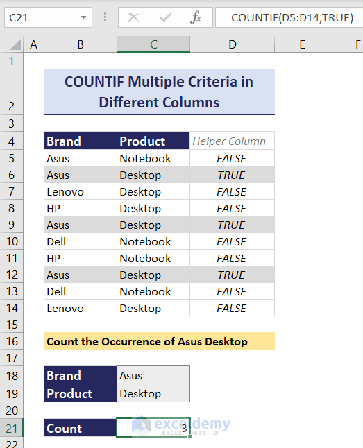
You want to count how many times Asus Desktop occurs. There are 2 criteria: the brand, Asus, and the type of product, a Desktop.
Overview of Using Excel COUNTIF with Helper Column Based on Multiple Criteria in Different Columns
- Create a helper column, column in D.
- Use the AND function to identify which brand-product pair is TRUE in the set criteria (Asus Desktop). Use the COUNTIF function to count occurrences: 3.
Example 1 – Matching 2 AND Type Criteria (HP Desktops) in Different Columns
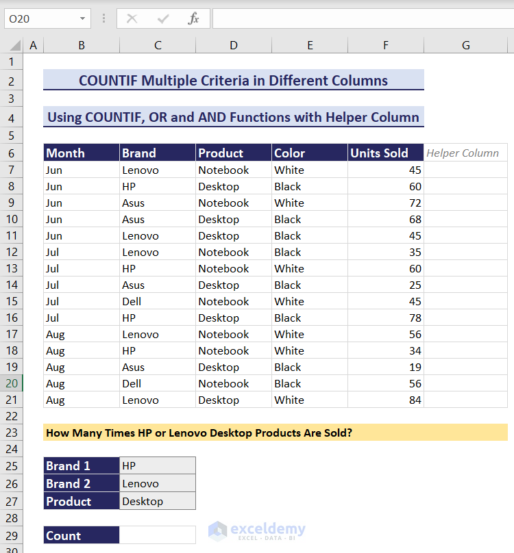
The sales dataset contains Month, Brand, Product, Color, and Units Sold.
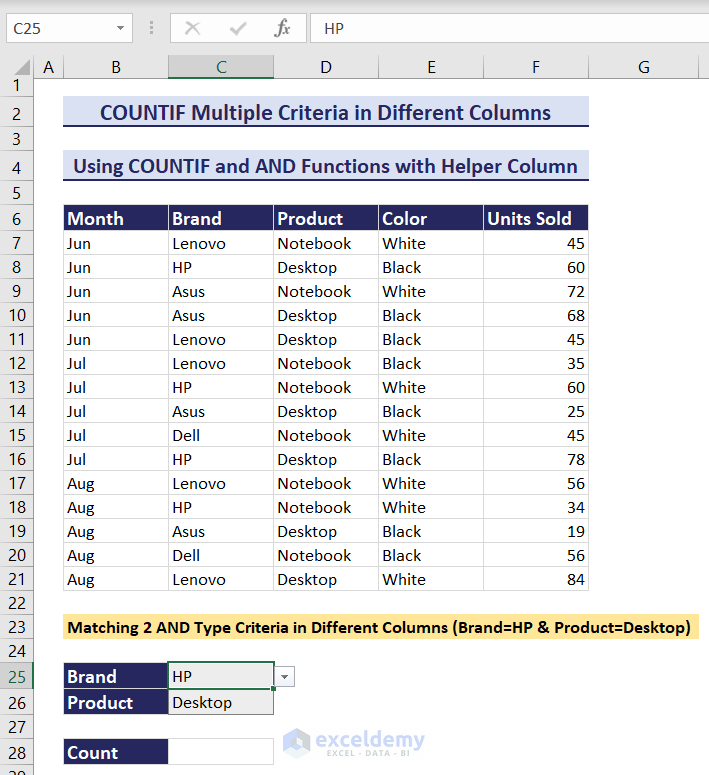
To count how many times the HP Desktop occurs:
The AND function has the following syntax:
=AND(logical1,[logical2], …)
Step 1:
- Add a helper column in G.
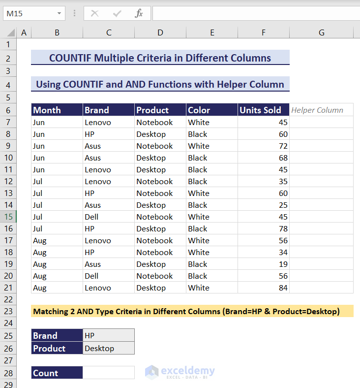
Step 2:
- The criteria are HP and Desktop.
- Enter this formula in G7:
=AND(C7=$C$25,D7=$C$26)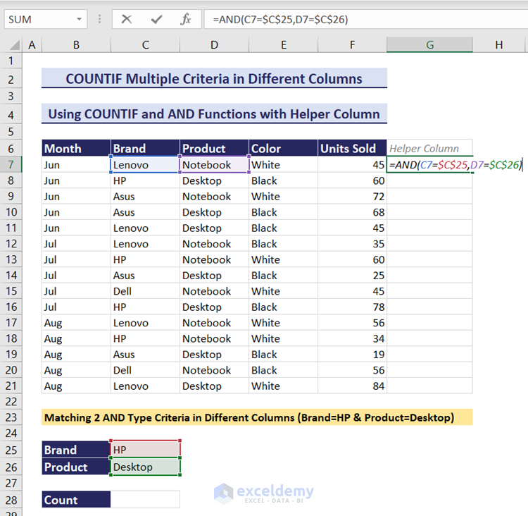
Step 3:
- Press Enter to see the output.
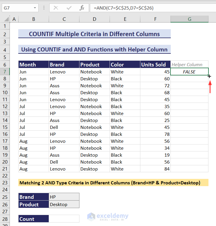
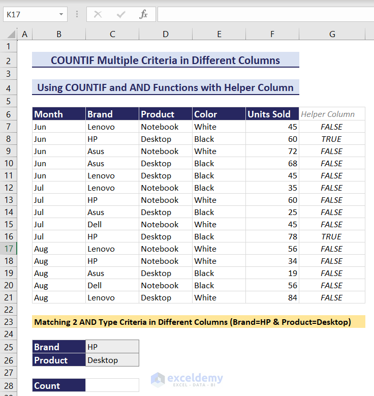
Step 4:
- Drag down the Fill Handle to see the result in the rest of the cells.
Step 5:
- In C28, count TRUE in G7:G21. Enter this formula in C28:
=COUNTIF(G7:G21,TRUE)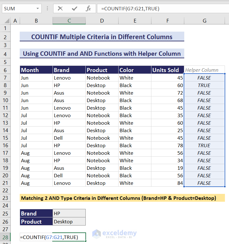
Step 6:
- Press the Enter to see the output.
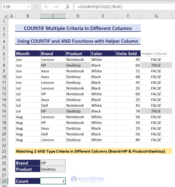
HP Desktop occurs twice.
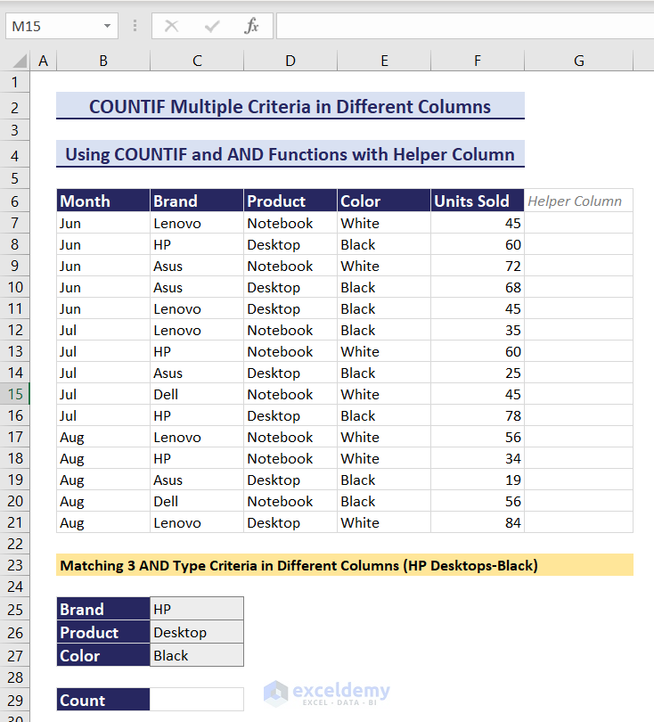
Example 2 – Matching 3 AND Type Criteria (Black HP Desktops) in Different Columns
To match 3 criteria (= HP, product = Desktop, and color = Black) and return the count:
Step 1:
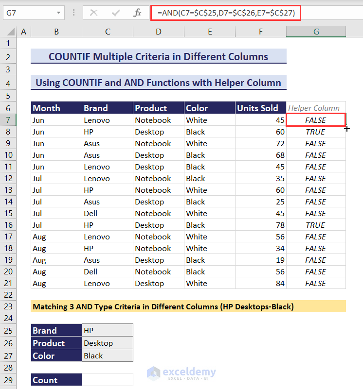
- In G7, enter this formula:
=AND(C7=$C$25,D7=$C$26,E7=$C$27)E7=$C$27 is the 3rd condition added (color=Black).
Step 2:
- Press the Enter to see the output.
Step 3:
- Use the formula below.
=COUNTIF(G7:G21,TRUE)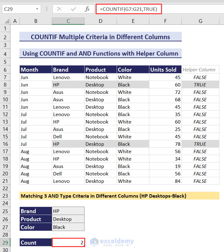
Black HP Desktop occurs twice.
Example 3 – How Many Times were HP or Lenovo Desktop Products Sold? (AND-OR Criteria Combination)
The syntax of the OR function is:
=OR(logical1,[logical2], …)
It returns TRUE if any of the conditions is true. If not a single criterion is true, it returns FALSE:
OR(TRUE,FALSE) = OR(FALSE,TRUE) = OR(TRUE,TRUE) = TRUE
But, OR(FALSE,FALSE) = FALSE
The formula is:
=OR(AND(brand_cell=HP,product_cell=Desktop),AND(brand_cell=Lenovo,product_cell=Desktop))
If any of the AND part of this formula returns TRUE, OR will return TRUE.
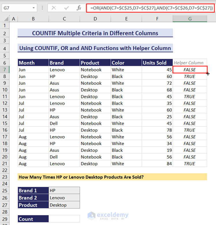
Step 1:
- In G7, enter this formula:
=OR(AND(C7=$C$25,D7=$C$27),AND(C7=$C$26,D7=$C$27))Step 2:
- Press the Enter to see the output.
Step 3:
- Use the COUNTIF formula.
=COUNTIF(G7:G21,TRUE)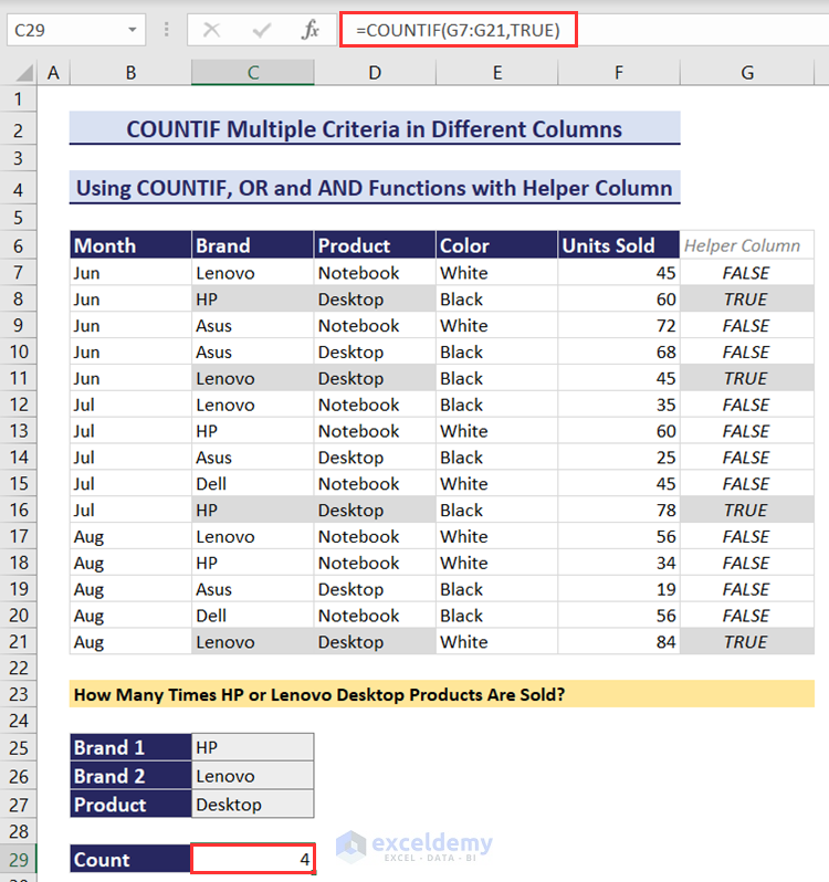
The HP or Lenovo Desktops occur 4 times.
Example 4 – How Many Times did HP Desktops sell More Than 40 Units?
The criteria are brand = HP, product = Desktop, and Units sold > 40.
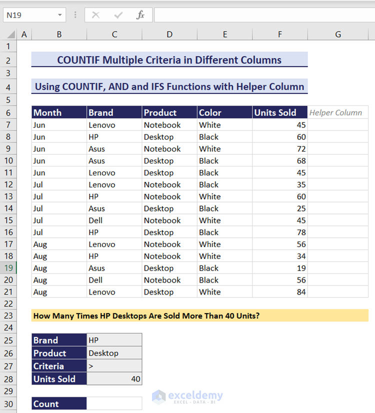
- Use the following formula to create a helper column in G.
=AND(C7=$C$25,D7=$C$26,F7>$C$28)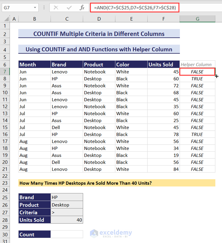
- Enter the following formula:
=COUNTIF(G7:G21,TRUE)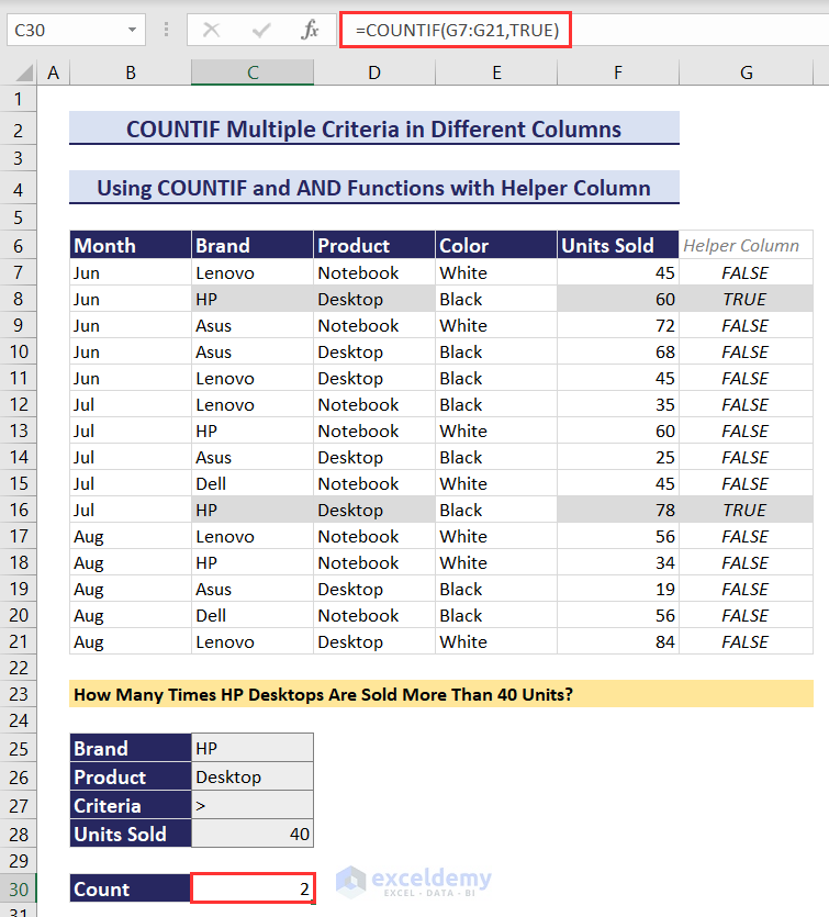
More than 40 units of HP Desktops are sold twice.
Modify the Formula in the Helper Column for Greater/ Less Than or Equal to Criteria:
Use the AND function in the helper column.
Divide the third criterion into 2 segments- one is greater than (>); the other is 40 (here).
Use the IFS function with the AND function to create the helper column.
The syntax of the IFS function is:
=IFS(logical_test1, value_if_true1, …)
The IFS function can check multiple conditions.
If the first condition is not TRUE, it checks whether the 2nd condition is TRUE. If the 2nd one is not TRUE, it checks the 3rd condition and so on.
It returns an assigned value for the first TRUE condition. If no condition is TRUE, then it returns FALSE or the assigned value for FALSE.
It does not check the next condition if the previous one is TRUE.
This function replaces nested IF functions.
- Enter the following formula in G7, press Enter, and drag down the Fill Handle:
=AND(C7=$C$25,D7=$C$26,IFS($C$27="=",F7=$C$28,$C$27=">=",F7>=$C$28,$C$27=">",F7>$C$28,$C$27="<=",F7<=$C$28,$C$27="<",F7<$C$28))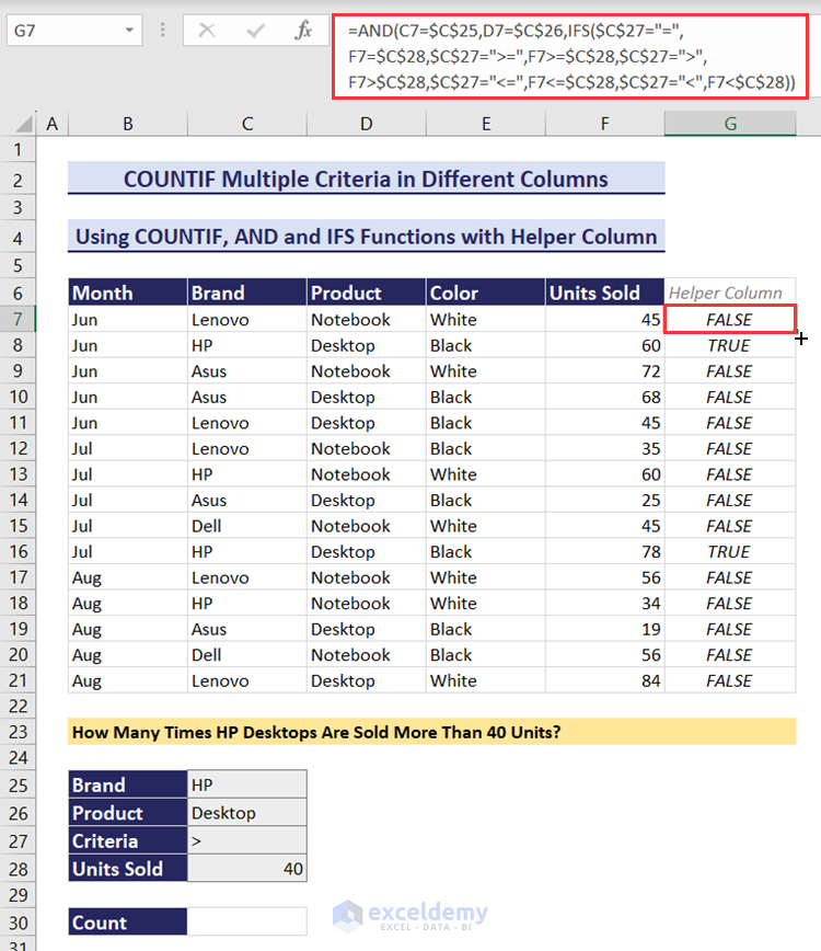
- Enter the following formula in C29 to count TRUE in G7:G21:
=COUNTIF(G7:G21,TRUE)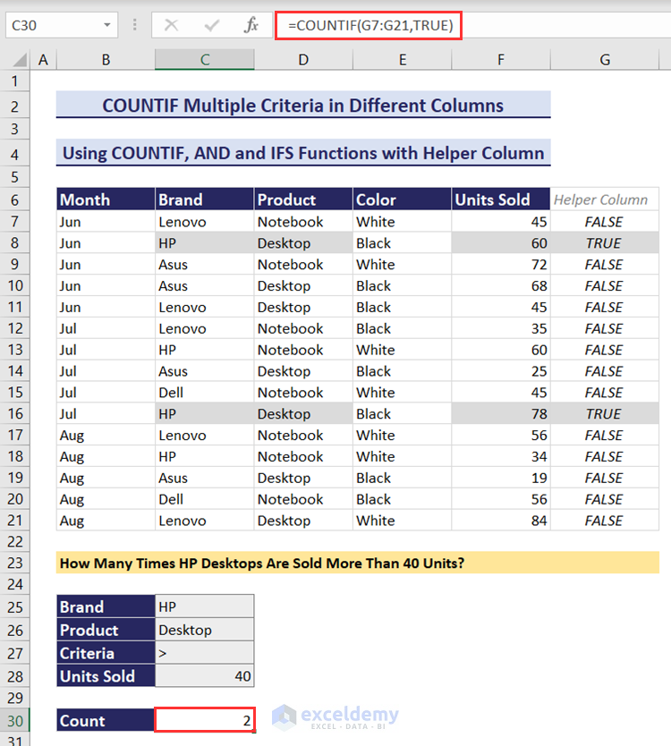
More than 40 units HP Desktops were sold twice.
Alternative 1 – Using the COUNTIFS Function with Multiple Criteria in Different Columns Instead of the COUNTIF
The Syntax of the COUNTIFS function is:
=COUNTIFS(criteria_range1, criteria1, [criteria_range2, criteria2]…)
Example 1 – Matching 2 AND Type Criteria (HP Desktops) in Different Columns
- To count how many times HP desktops occurs, use the following formula in C28.
=COUNTIFS(C7:C21,C25,D7:D21,C26)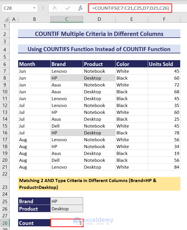
Example 2 – Matching 3 AND Type Criteria (Black HP Desktops) in Different Columns
- Modify the previous COUNITFS formula:
=COUNTIFS(C7:C21,C25,D7:D21,C26,E7:E21,C27)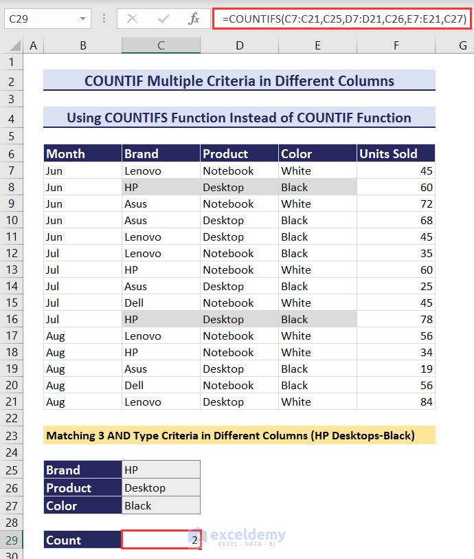
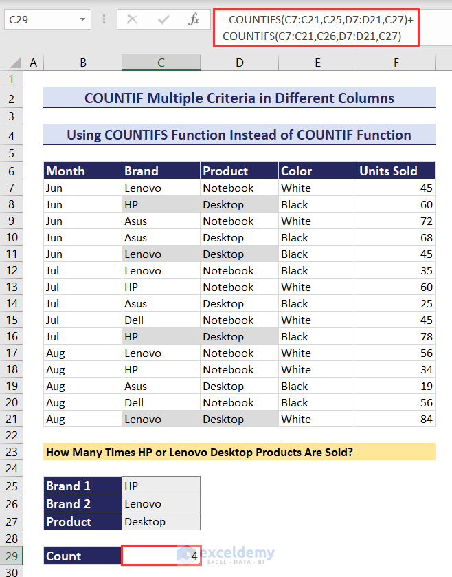
Example 3 – How Many Times Are HP or Lenovo Desktop Products Sold? (AND-OR Criteria Combination)
- Enter the following formula in C29:
=COUNTIFS(C7:C21,C25,D7:D21,C27)+COUNTIFS(C7:C21,C26,D7:D21,C27)COUNTIFS(C7:C21,C25,D7:D21,C27) returns the count of HP Desktops.
And COUNTIFS(C7:C21,C26,D7:D21,C27) returns the count of Lenovo Desktops.
The plus operator is the OR criteria.
Example 4 – How Many Times did HP Desktops Sell More Than 40 Units?
The criteria are brand = HP, product = Desktop, and Units sold > 40.
- Enter this formula in C30:
=COUNTIFS(C7:C21,C25,D7:D21,C26,F7:F21,C27&C28)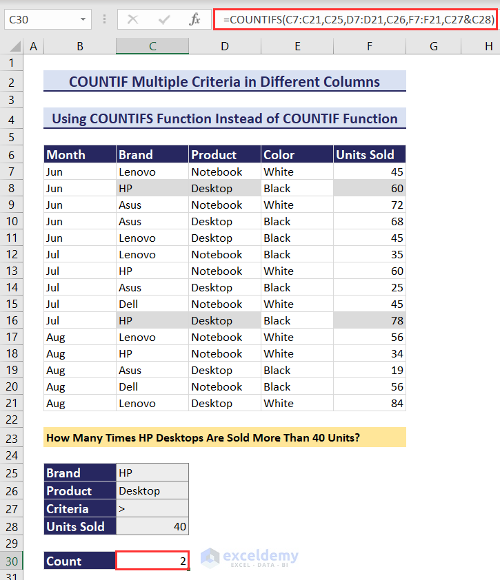
Alternative 2 – Using the SUMPRODUCT Function in Excel 2007 or Later Versions
The syntax of the SUMPRODUCT function is:
=SUMPRODUCT(array1, [array2], [array3], …)
It returns the sum of the products of given ranges or arrays. The arrays should have the same number of rows and columns.
This function can be used in all the above-mentioned examples.
- In Example 1, the SUMPRODUCT formula will be the following:
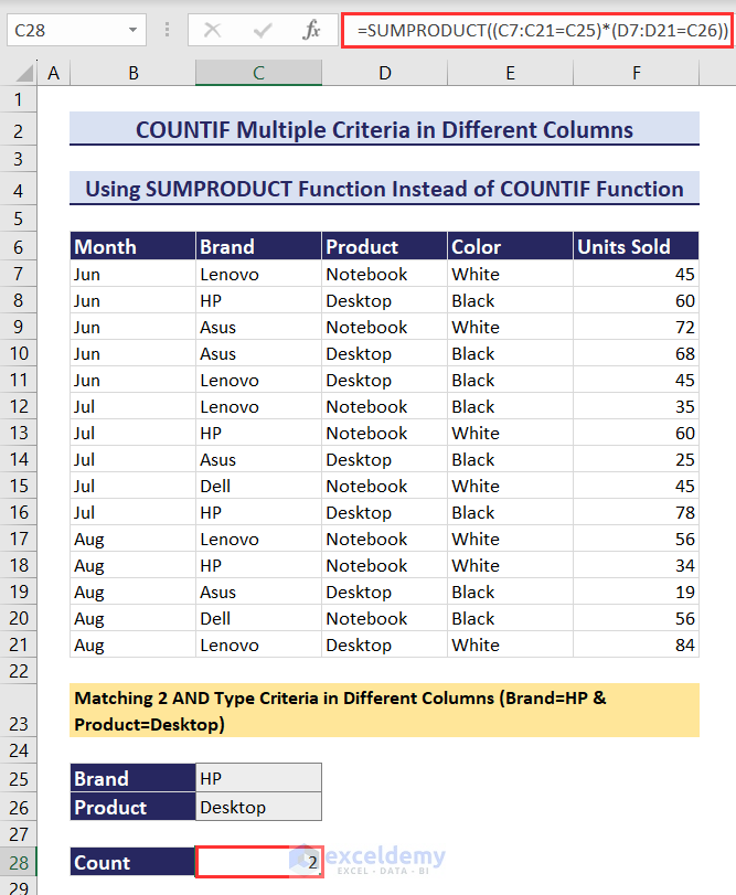
=SUMPRODUCT((C7:C21=C25)*(D7:D21=C26))In Example 2:
=SUMPRODUCT((C7:C21=C23)*(D7:D21=C25)*(E7:E21=C26))In Example 3:
=SUMPRODUCT(((C7:C21=C23)+(C7:C21=C24))*(D7:D21=C25))In Example 4:
=SUMPRODUCT((C7:C21=C23)*(D7:D21=C25)*(IFS($C$27="=",F7:F21=$C$28,$C$27=">=",F7:F21>=$C$28,$C$27=">",F7:F21>$C$28,$C$27="<=",F7:F21<=$C$28,$C$27="<",F7:F21<$C$28)))
Read More: SUMPRODUCT and COUNTIF functions with multiple criteria
Alternative 3: Use the SUM Function Instead of the COUNTIF with a Helper Column (Available in All Excel Versions)
- In Example 1, the formula is:
=SUM((C7:C21=C25)*(D7:D21=C26))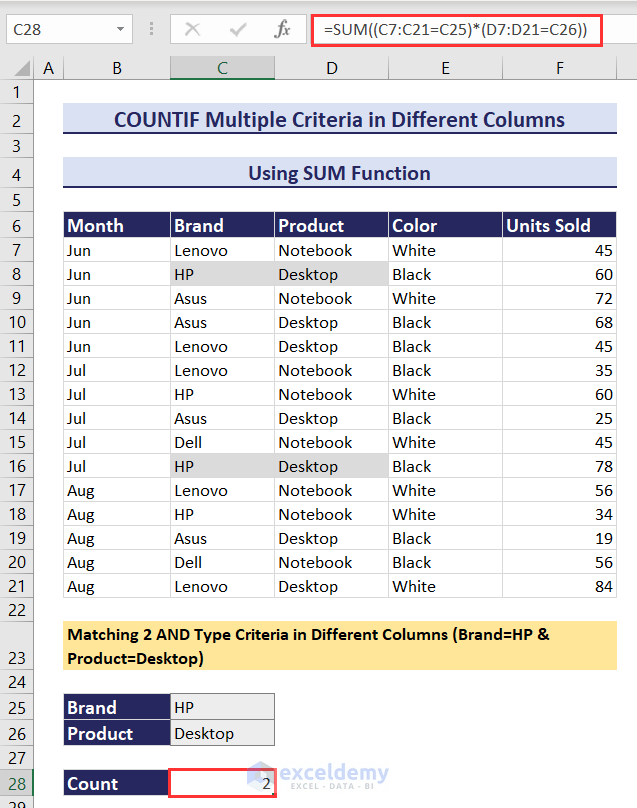
In Example 2:
=SUM((C7:C21=C23)*(D7:D21=C25)*(E7:E21=C26))In Example 3:
=SUM(((C7:C21=C23)+(C7:C21=C24))*(D7:D21=C25))In Example 4:
=SUM((C7:C21=C23)*(D7:D21=C25)*(IFS($C$27="=",F7:F21=$C$28,$C$27=">=",F7:F21>=$C$28,$C$27=">",F7:F21>$C$28,$C$27="<=",F7:F21<=$C$28,$C$27="<",F7:F21<$C$28)))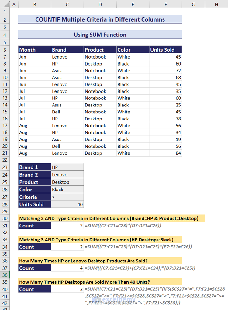
Download Practice Workbook
Related Articles
- COUNTIF Between Two Values with Multiple Criteria in Excel
- How to Use COUNTIF Between Two Dates and Matching Criteria in Excel
- Excel COUNTIF Function with Multiple Criteria & Date Range
- How to Use COUNTIF with Multiple Criteria in the Same Column in Excel
- How to Use COUNTIF for Cells Not Equal to Text or Blank in Excel
- How to Apply SUM and COUNTIF for Multiple Criteria in Excel
- How to Use COUNTIF Function Across Multiple Sheets in Excel
<< Go Back to COUNTIF Multiple Criteria | Excel COUNTIF Function | Excel Functions | Learn Excel
Get FREE Advanced Excel Exercises with Solutions!

I need count one criteria in (A1:A10,”TOM”) & Count how many in C1:C10
COLUMN A feild “NAME”
COLUMN C Field in No of “BL” ANSWER= 5
A C
TOM 2
ANN 1
TOM 1
ABI 2
ANN 2
TOM 2
Thank you ZOYSA for your comment. Below, I have attached two formulas for your problem.
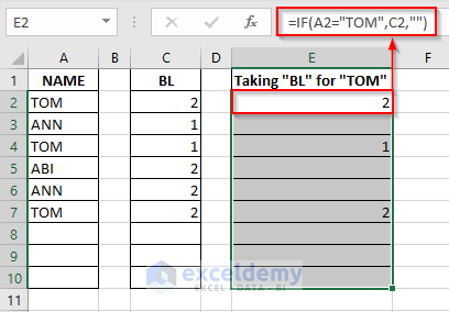
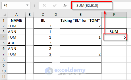
I have written the data from the A2 cell and C2 cell. According to your question, I have considered the dataset till A10 and C10.
Firstly, write the below formula in the E2 cell or the cell from where the NAME will be started.
=IF(A2=”TOM”,C2,””)
Then copy this formula up to E10 or your dataset’s end cell.
Then use another formula in the F4 cell.
=SUM(E2:E10)