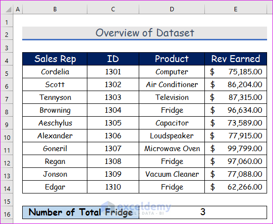
SUMPRODUCT and COUNTIF Functions with Multiple Criteria

The sample dataset contains the record of the product, sales representative names, their ID, and revenue earned by those sales representatives.

sumproduct countif multiple criteria

Example 1 – Combine SUMPRODUCT and COUNTIF Functions to Count Cells Between Numbers

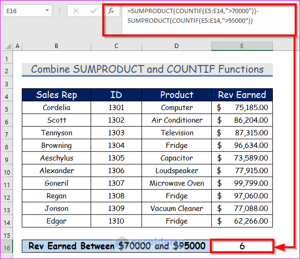
To find the total number of sales representatives whose revenue earned falls between $70000 and $95000,

Steps:

In the cell E16, enter the following SUMPRODUCT and COUNTIF functions.

=SUMPRODUCT(COUNTIF(E5:E14,">70000"))-SUMPRODUCT(COUNTIF(E5:E14,">95000"))

Formula Breakdown:

SUMPRODUCT(COUNTIF(E5:E14,”>70000″)) will count cells greater than 70000.
SUMPRODUCT(COUNTIF(E5:E14,”>95000″)) will count cells less than 95000.
The above formula will find cells for 70000< cells < 95000.

Press Enter. It will display the total number of sales representatives whose revenue earned falls between $70000 and $95000, which is 6.

Example 2 – Applying SUMPRODUCT and COUNTIF Functions with Multiple Criteria for Text in Same Column

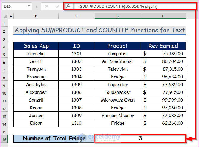
To find the number of Fridge in a single column,

Steps:

Enter the following SUMPRODUCT and COUNTIF functions in cell D16.

=SUMPRODUCT(COUNTIF(D5:D14,"Fridge"))

Formula Breakdown:

D5:D14 is the range and “Fridge” is the criteria of the COUNTIF function.
COUNTIF(D5:D14,”Fridge”) is the array of the SUMPRODUCT function.

Press Enter. You will get the total number of the Fridge in the column, which is 3.

Similar Readings

Example 3 – Utilizing SUMPRODUCT and COUNTIF Functions with Multiple Criteria for Dates

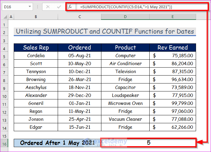
To count the cells whose product was ordered after May 1, 2021.

Steps:

Enter the following functions in cell D16.

=SUMPRODUCT(COUNTIF(C5:D14,">1 May 2021"))

Formula Breakdown:

C5:D14 is the range and “>1 May 2021” is the criteria of the COUNTIF function.
COUNTIF(C5:D14,”>1 May 2021″) is the array of the SUMPRODUCT function.

Press Enter. The output is 5.

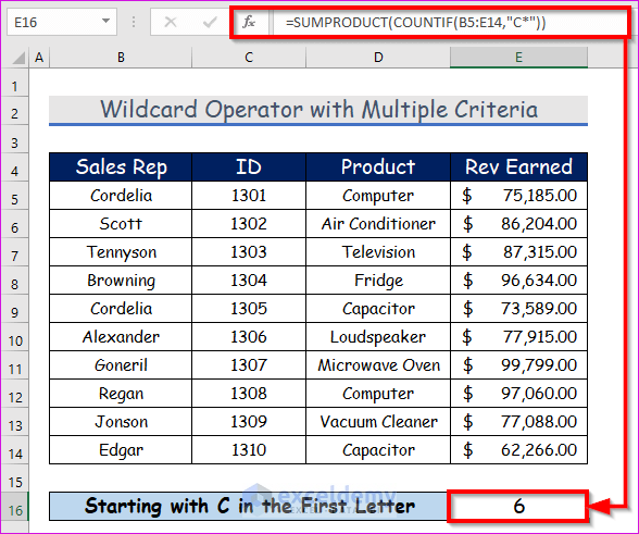
Example 4 – Wildcard Operator with Multiple Criteria in Multiple Columns

We will apply the wildcard operator in the SUMPRODUCT and COUNTIF functions to count the specific cells. There are 3 wildcard characters that are used in Excel.

Asterisk (*) – It searches any number of characters after a text.

Question Mark (?) – This question mark is used to replace a single character.

Tilde (~) – It can nullify the impact of the above two characters.

We will count the sales representatives and products whose names start with the C.

Steps:

Enter the following functions in the cell E16.

=SUMPRODUCT(COUNTIF(B5:E14,"C*"))

Formula Breakdown:

B5:E14 is the range and “C*” is the criteria of the COUNTIF function.
COUNTIF(B5:E14,”C*”) is the array of the SUMPRODUCT function.