How to Use COUNTIFS Between Two Dates and Matching Criteria in Excel

The COUNTF function counts data based on a single criterion. But when multiple ranges and matching criteria are involved, we can use its alternative, the COUNTIFS function.

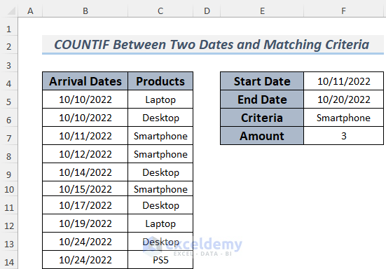
In the dataset below, we have the Arrival Dates of some electronic devices. Let’s use COUNTIFS to count how many of a specific item arrived within a specified date range.

Method 1 Using Excel COUNTIFS Function Between Two Dates and Matching Criteria

Let’s count how many Smartphones arrived in the store between 11th and 20th October.

Steps:

Select some cells to define the date range and set the criteria. Here, the Start and End Dates will be 11th and 20th October, and our criteria is Smartphone which we will match with the data in the Products column.
Select another cell to count the items – here cell F7 – and enter the following formula in it:

=COUNTIFS($B$5:$B$14,">="&F4,$B$5:$B$14,"<="&F5,C5:C14,F6)

Press ENTER.

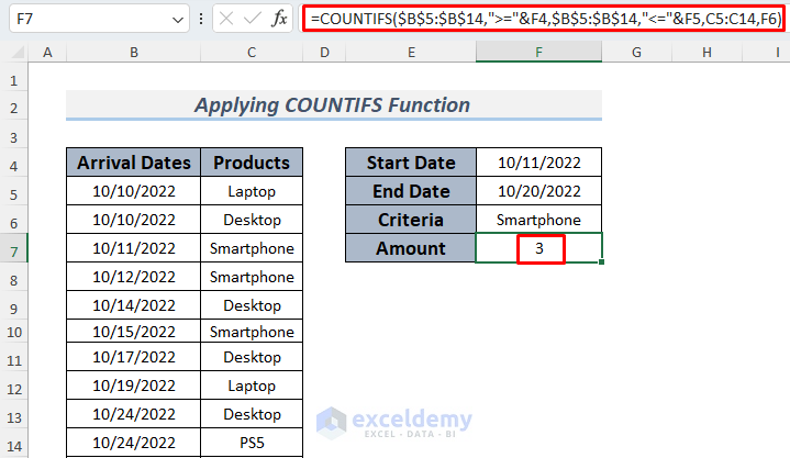
Here, our date range is between the 11th and 20th October. So the first criterion is that the date in the date range has to be greater than or equal to the 11th October. Similarly, the second criterion is that the date should be less than or equal to the 20th October. As the first and second criteria are dates, we select the date range (Arrival Dates) column (B5:B14). We set the matching criteria in cell F6 which we find in the Products column. So the Criteria Range is C5:C14 and the Criteria is F6. As the Smartphones arrived three times in that period, the formula will return 3.

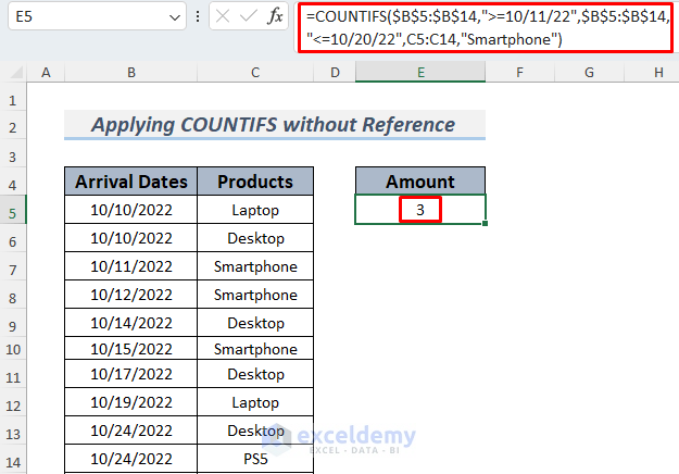
Method 2 – Using the COUNTIFS Function Without Cell Reference

We can also hard code the two dates (Starting and Ending) and the criteria (Smartphone) in the formula to get the same result as in Method 1.

Steps:

Select a cell to count the items (E3) and enter the following formula in it:

=COUNTIFS($B$5:$B$14,">=10/11/22",$B$5:$B$14,"<=10/20/22",C5:C14,"Smartphone")

Press ENTER.

The operation will return the number of Smartphones that arrived between 11th and 20th October.

Inserting the date period and criteria manually requires less complexity, but it is time costly and not an efficient procedure. Using cell references would therefore generally be the better choice.

Method 3 – Combining EOMONTH Function with COUNTIFS Between Two Dates and Matching Criteria

In this method, we will select the End Date by using the EOMONTH function.

Steps:

Select some cells to define the date range and set the criteria. The Start and End Dates will be the 11th and 31st October.
Set the last date of the month with the following formula:

=EOMONTH(F4,0)

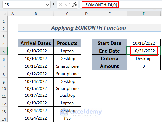
The EOMONTH function returns the last date of the corresponding month if the second argument in the formula is 0. If the second argument is 1, then it will return the last date of the next month. Similarly, for 2, 3, 4, and so on, it will add one month respectively.

In addition, our criteria here is Desktop which we will match with the data in the Products column.

Select another cell to count the items (F7) and enter the following formula in it, then press ENTER:

=COUNTIFS($B$5:$B$14,">="&F4,$B$5:$B$14,"<="&F5,C5:C14,F6)

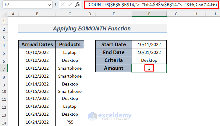
Our time frame in this case is from October 11 to October 20. Therefore the first requirement is that the date within the range must be greater than or equal to October 11th. The second requirement is that the date must be less than or equal to October 20. We choose the date range (Arrival Dates) column because the first and second criteria are dates (B5:B14). The matching criteria are entered in cell F6, and the Products column contains the results. Therefore, the next set of criteria has a range of C5:C14 and an F6 standard. The formula will count 3 because the Desktop arrived 3 times throughout the specified time.

Similar Reading

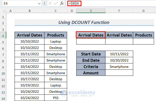
Useful Alternative: Using DCOUNTA and SUMPRODUCT Functions Between Two Dates and Matching Criteria

Case 1 – Using the DCOUNTA Function

Steps:

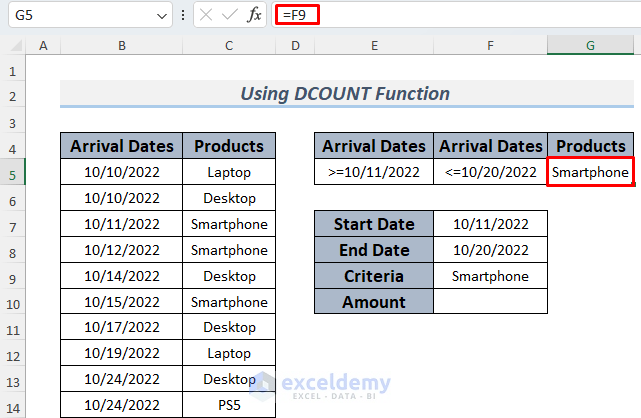
Enter the cell value of cell B4 in cell E5 by using the formula below:

=$B$4

Enter the formula below in cell E5 and press ENTER.

=">="&TEXT(F7,"m/d/yyy")

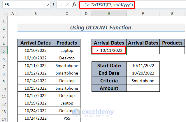
The formula uses the TEXT function to set up the Start Date criteria for the DCOUNTA function.

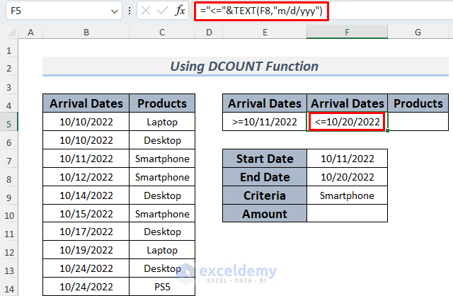
Enter the formula below to set up the End Date:

="<="&TEXT(F8,"m/d/yyy")

Insert the cell value of cell F9 in cell G5 using the following formula, which is the match criteria for the DCOUNTA function:

=F9

Enter the following formula in cell F10:

=DCOUNTA(B4:C14,G4,E4:G5)

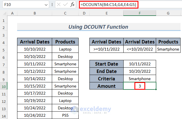
The DCOUNTA function works on a database, which here is the entire dataset of products and their arrival dates (B4:C14), the first argument of this function. The second argument is the field argument which is the product type referred to by cell G4. The final argument here is the criteria, which is the range E4:G5. The formula will return 3 as the Smartphones have arrived 3 times in this period.

Case 2 – Using the SUMPRODUCT Function

Steps:

Select some cells to define the date range and set the criteria. The Start and End Dates will be 11th and 20th October. Our criteria here is Smartphone, which we will match with the data in the Products column.
Select another cell to count the items (F7) and enter the following formula in it, then press ENTER:

=SUMPRODUCT(--($B$5:$B$14>=F4),--($B$5:$B$14<=F5),--(C5:C14=F6))

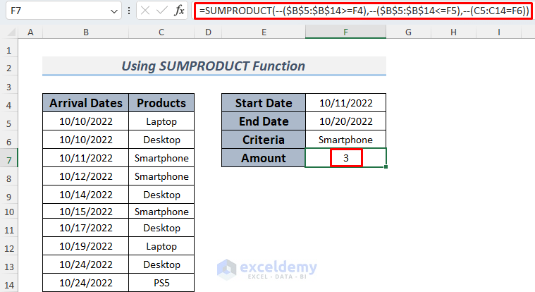
Formula Breakdown

The formula uses the sum of products of some logical values, which are obtained from the comparison between the dates and criteria (Smartphone).

–($B$5:$B$14>=F4) —-> returns an array with ones and zeros.
- Output: {0;0;1;1;1;1;1;1;1;1}
–($B$5:$B$14<=F5) —-> returns a similar array.
- Output: {1;1;1;1;1;1;1;1;0;0}
–(C5:C14=F6) —-> will become
- Output: {0;0;1;1;0;1;0;0;0;0}
The formula turns into
=SUMPRODUCT({0;0;1;1;1;1;1;1;1;1}, {1;1;1;1;1;1;1;1;0;0}, {0;0;1;1;0;1;0;0;0;0}) —-> which returns
- Output: 3