How to Hide Zero Values in Excel Pie Chart (3 Simple Methods)

Get FREE Advanced Excel Exercises with Solutions!

Excel is the most widely used tool for dealing with massive datasets. We can perform myriads of tasks of multiple dimensions in Excel. Sometimes, we need to show information in charts for our convenience. This not only helps understand a report better but also makes the report look exquisite. Pie charts are good options to represent data in graphical form. But often we have zero values in pie charts which we want to get rid of. In this article, I will show how to hide zero values in Excel Pie Chart.

Table of Contents hide

Download Practice Workbook

3 Simple Methods to Hide Zero Values in Pie Chart in Excel

1. Use Filter Feature to Hide Zero Values in Excel Pie Chart

2. Create Table to Hide Zero Values in Excel Pie Chart

3. Format Data Labels to Hide Zero Values in Excel Pie Chart

Things to Remember

Conclusion

Download Practice Workbook

Download this workbook and practice while going through the article.

Hide Zero from Pie Chart.xlsx

3 Simple Methods to Hide Zero Values in Pie Chart in Excel

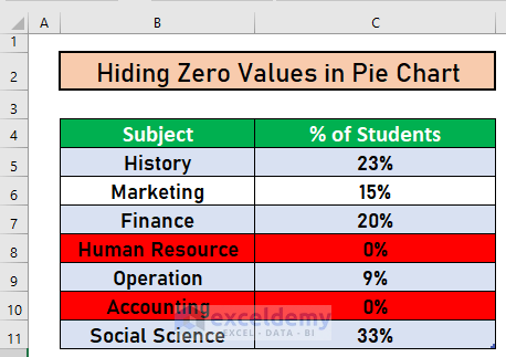
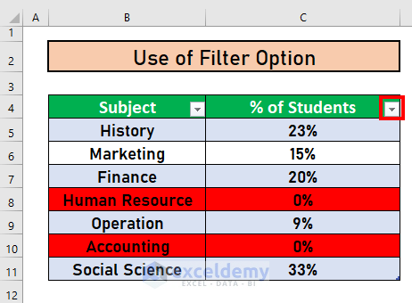
This is the dataset for today’s article. There are some major subjects and the number of students who have taken them respectively. Notice that, no students have taken Human Resource and Accounting. Now, I am going to prepare a pie chart hiding these values.

1. Use Filter Feature to Hide Zero Values in Excel Pie Chart

The first method is the use of the Filter Option in Excel. In this method, we will filter the zero values to hide them. Let’s do this step by step.

Steps:

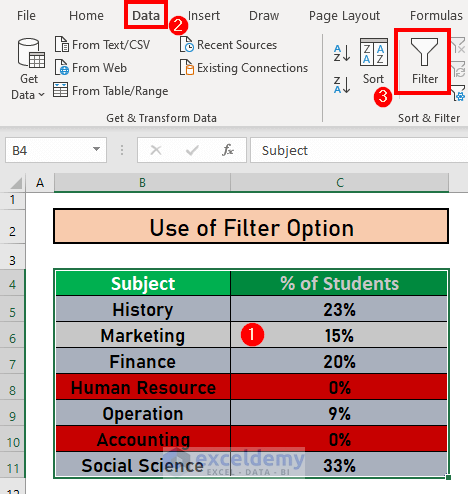
First of all, select the entire dataset.
Then, go to the Data.
After that, select Filter.

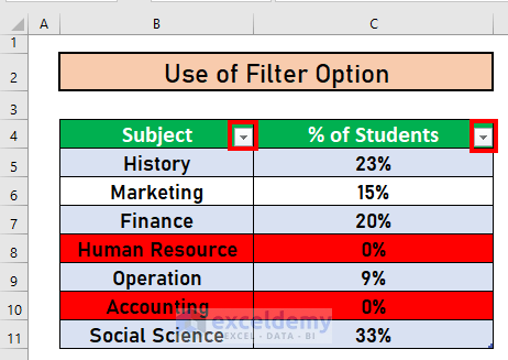
You will see that Excel has added the Filter Excel will create drop-down lists for each column.

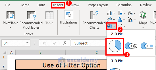
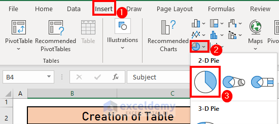
Now, you have to insert the pie chart. To do so,

Go to the Insert.
Then, select the pie charts. Excel will show the available ones.
After that, select the one you find suitable. I am going to select the 2-D.

Excel will create the pie chart. However, you will see that the Human Resource and Accounting subjects are still there in the Legend.

We will hide these subjects with 0%. To do so,

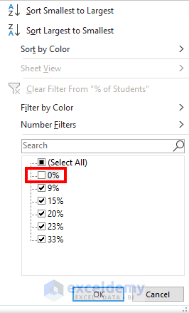
Select the drop-down box for the column % of Students.

Then, uncheck the box for 0.

Excel will hide the zero values from the pie chart.

Similar Readings

2. Create Table to Hide Zero Values in Excel Pie Chart

Now, I will discuss another method to hide zero values in Excel pie charts. We will create a table in this method instead of applying Filter. The rest is similar to method-1.

Steps:

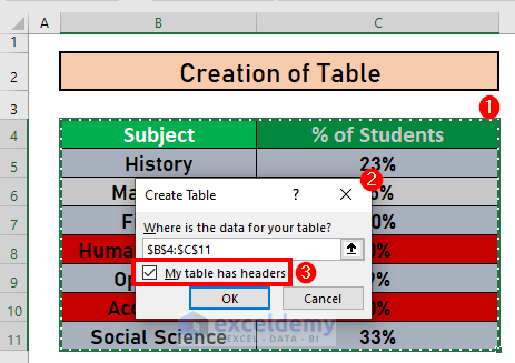
First of all, select the entire dataset.
Then, press CTRL+T to bring the Create Table.
Check the box for My table has headers since there are headers in the columns.
Finally, click OK.

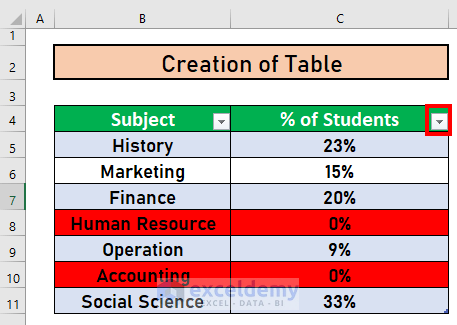
Excel will create a table. You will notice that Excel has also applied the Filter option in the table.

Now, you have to insert the pie chart. To do so,

Go to the Insert.
Then, select the pie charts. Excel will show the available ones.
After that, select the one you find suitable. I am going to select the 2-D.

Excel will create the pie chart. However, you will see that the Human Resource and Accounting subjects are still there in the Legend.

We will hide these subjects with 0%. To do so,

Select the drop-down box for the column % of Students.

Then, uncheck the box for 0.

Excel will hide the zero values from the pie chart.

3. Format Data Labels to Hide Zero Values in Excel Pie Chart

In this section, I will discuss another method to hide zero values from pie charts. This time, I will not use any Filter. Rather, I will format data labels to hide zeroes.

Steps:

First of all, insert a pie chart following method-1.

After that, right-click your mouse to bring up the menu.
Then, select Add Data Labels.

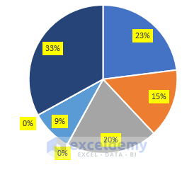
Excel will add data labels.

Now, I will slightly modify the data labels to make them look clearer. For this,

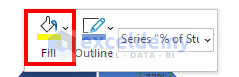
Select the data labels.
Then, change the Fill color.

Excel will change the Fill color. Notice that there are two 0% values.

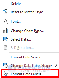
I will now hide these 0% values. To do so,

Select the Data labels.

Then, right-click your mouse to bring the menu.
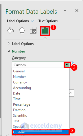
After that, select Format Data Labels.

Now, go to Label Options.
Then, select the Number Category as Custom.

After that, write the following format,

0.00%;;;

Finally, click Add.

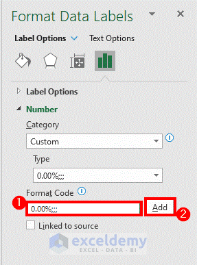
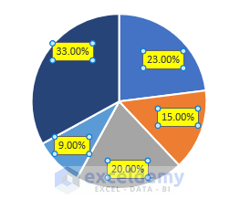
Excel will hide the zero values. The final output will be like this.

Things to Remember

You have to filter the dataset. Otherwise, Excel will not hide the category.
You can even draw a 3D pie chart if you wish.
Hiding zero value will keep your report short and succinct.
When you format data labels, the categories having zero values will remain in the Legend.

Conclusion

In this article, I have demonstrated 3 easy methods on how to hide zero values in Excel Pie Charts. I hope it helps everyone. If you have any suggestions, ideas, or feedback, please feel free to comment below. Please visit Exceldemy for more valuable articles like this.