How to Explode a Pie Chart in Excel – 2 Methods

This is the sample dataset.

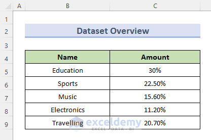
This is the corresponding pie chart:

Method 1 – Exploding a Pie Chart Using the Mouse Cursor

Steps:

• Select the pie chart.

• Drag a portion away from the pie. Here, Traveling.

• Drop the portion away from the pie.

To explode multiple portions, repeat the process. Here, Traveling, Music, and Electronics.

Read More: How to Edit Pie Chart in Excel

Method 2 – Use the Format Data Series Option to Explode a Pie Chart

Steps:

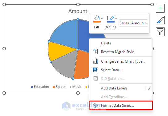
• Select the pie chart and right-click it.
• Select Format Data Series.

• The Format Data Series panel will be displayed.

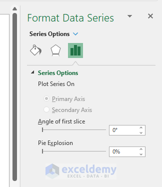
• Select Pie Explosion.

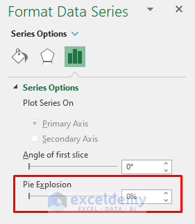
• Set Pie Explosion to different values. Here, to 20%.

Read More: How to Rotate Pie Chart in Excel

Things to Remember

• Exploding Pie Charts by Dragging the Cursor scatters the plot portions unevenly.
• Higher percentage values in Pie Explosion may result in shortening the pie portions to maintain distance in the specific chart area.
• These methods are also applicable to 3-D Pie charts.

Download Practice Workbook

Related Articles

• How to Change Pie Chart Colors in Excel
• How to Edit Legend of a Pie Chart in Excel
• Add Labels with Lines in an Excel Pie Chart
• [Fixed] Excel Pie Chart Leader Lines Not Showing
• How to Hide Zero Values in Excel Pie Chart
• Excel Pie Chart Labels on Slices: Add, Show & Modify Factors

<< Go Back To Edit Pie Chart in Excel | Excel Pie Chart | Excel Charts | Learn Excel