Method 1 – Use Fill Color Tool to Change Pie Chart Colors
- Double-click on any of the slices in the pie chart.

- Right-click and select Fill.
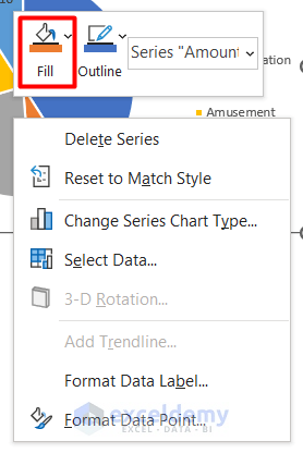
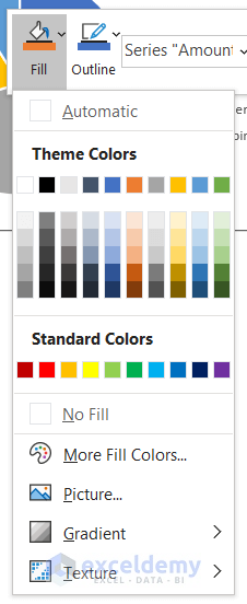
- Select any color for the slice.
- The slice will change to the selected color.

- Change other slice colors by following the same procedure.
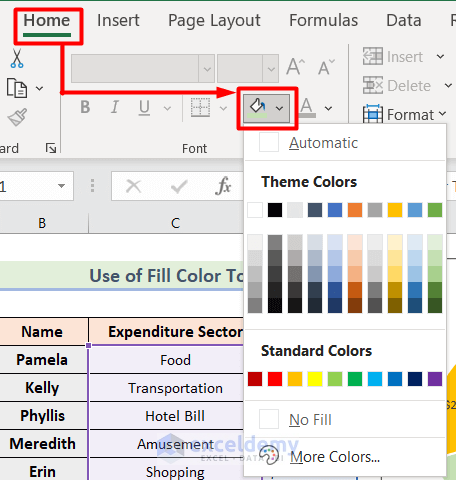
- Fill Color tool is in the Font group of the Home tab.
- Select More Colors.

- The Colors window will open where you can customize colors as desired.

Method 2 – Apply Themes in Excel to Modify Pie Chart Colors
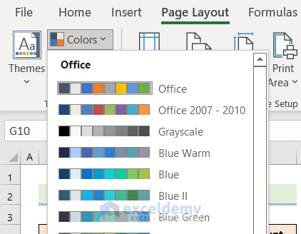
- Select Colors in the Themes group of the Page Layout tab.
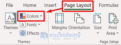
- Choose a color set.
- The slice colors will change.

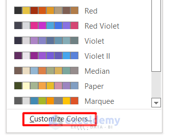
- To edit any color of the selected color set, go to Customize Colors.
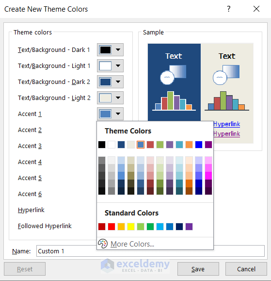
- In the Create New Theme Colors window, change colors as desired.
- Click on Save.
Read More: How to Edit Legend of a Pie Chart in Excel
Method 3 – Change Pie Chart Colors in Excel with Chart Style
- Go to Page Layout tab and choose Change Colors from the Chart Styles group.
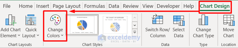
- Select the color from the options.
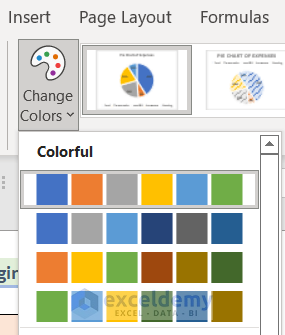
- The pie chart color will change.

- To change the background color,
- Click on Shape Fill under the Shape Styles group from the Format tab.
- Select any color.
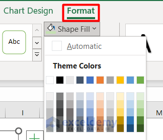
- Backgrund will change to the selected color.

Read More: How to Edit Pie Chart in Excel
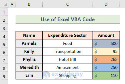
Method 4 – Use Excel VBA Code to Change Pie Chart Colors
- Color the cells D5:D9 manually with the Fill Color tool.
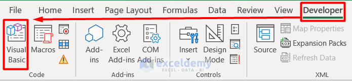
- Go to the Developer tab and select Visual Basic.
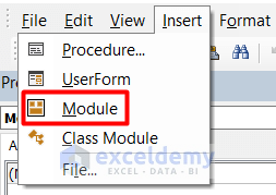
- In the visual basic window, Go to the Insert tab and select Module.
- Insert the code below on the blank page.
Private Sub SheetActivate()
    Dim ch As ChartObject
    Dim l As Long
    Dim vntValues As Variant
    Dim st As String
    Dim myS As Series

    For Each ch In ActiveSheet.ChartObjects

        For Each myS In ch.Chart.SeriesCollection

            If myS.ChartType <> xlPie Then GoTo SkipNotPie

            s = Split(myS.Formula, ",")(2)
            vntValues = myS.Values

            For l = 1 To UBound(vntValues)
                myS.Points(l).Interior.Color = Range(s).Cells(l).Interior.Color
            Next l
SkipNotPie:
        Next myS
    Next ch
End Sub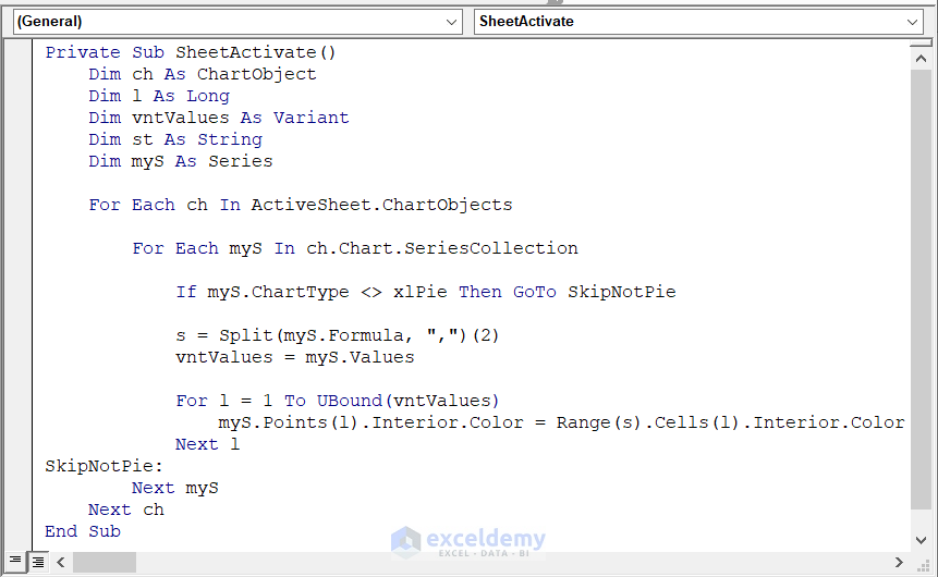
- Click on the Run Sub button or press F5 on your keyboard.
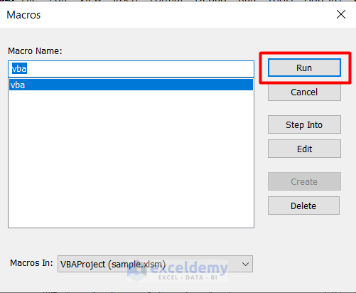
- Click on Run in the Macros window.
- The pie chart color will change.

Read More: Excel Pie Chart Labels on Slices: Add, Show & Modify Factors
How to Format Pie Chart Color in Excel
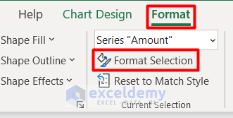
- Double-click on any slice of your pie chart.
- Select Format Selection in the Current Selection group under the Format tab.
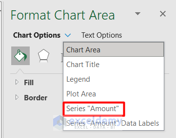
- In the Format Chart Area pane, go to Chart Options and select Series “Amount”.
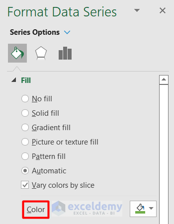
- Change the Color from this section.
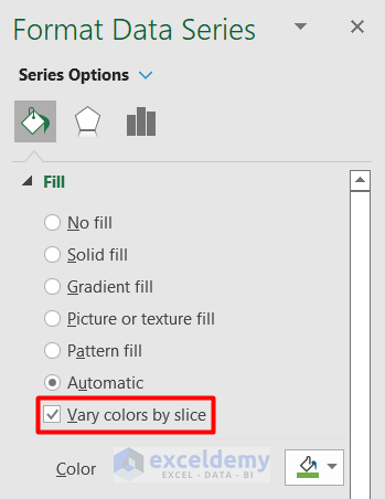
- Keep the Vary colors by slice option checked if you want different colors in each slice.
- Keep it unchecked to keep all the colors the same.
- Explore the Format Chart Area pane for more pie chart modification options.
Read More: Add Labels with Lines in an Excel Pie Chart
Download Workbook
Related Articles
- How to Rotate Pie Chart in Excel
- How to Explode Pie Chart in Excel
- [Fixed] Excel Pie Chart Leader Lines Not Showing
- How to Hide Zero Values in Excel Pie Chart
<< Go Back To Edit Pie Chart in Excel | Excel Pie Chart | Excel Charts | Learn Excel
Get FREE Advanced Excel Exercises with Solutions!
