How to Create Activity Relationship Chart in Excel

Are you an Industrial Production Engineer? Or do you have an interest in supply chain, system, and production engineering? Then, fasten the seat belt because there will be a bang now. In this article, we’ll demonstrate 4 easy and detailed steps to create an Activity Relationship Chart in Excel. So, let’s go through the article to perform the task efficiently in your work.

Introduction to Activity Relationship Chart

Designing the arrangement of the amenities that already exist on the production floor in order to maximize their productivity is known as facility layout. These resources could be tools, personnel, spaces, etc. For increased output, all of the assets must be appropriately organized on the shop floor. The foundation for creating any form of plant layout is an Activity Relationship Chart. For this chart to provide a useful plant layout, extreme care must be taken in its design.

What is Activity Relationship Chart?

An Activity Relationship Chart is also known as ARC in short. It’s in a tabular form to express the closeness rating between all sets of activities or departments. Each pair of departments in an ARC may be given one of the six closeness ratings, with nine justifications for each rating (each is assigned by a reason code).

Closeness Rating and Basis of the Coding in Activity Relationship Chart

The relationship chart shows which entities are connected to one another and assesses how important that connection is. The ratings and their closeness are given below.

Also, there are some reasons behind this closeness. We express them through number codes. So, you can see them below.

Importance of Activity Relationship Chart

The primary goal of the Activity Relationship Chart is to guarantee that the facility you are developing has the shortest possible distance between two pieces of equipment or departments that are crucial to one another. If the prior activity hasn’t been completed, no other activities can be performed. Imagine if you assigned a metal object to paint first, then welding, as opposed to welding first, then painting? Therefore, putting facilities closer together and shortening cycle times are the main goals.

How to Create Activity Relationship Chart in Excel: 4 Steps

In this section, we’ll learn the 4 basic steps to create an Activity Relationship Chart in Excel. So, let’s go through them one by one.
Here, we have used Microsoft Excel 365 version, you may use any other version according to your convenience. Don’t forget to inform us if you face any trouble while using any other versions of Excel.

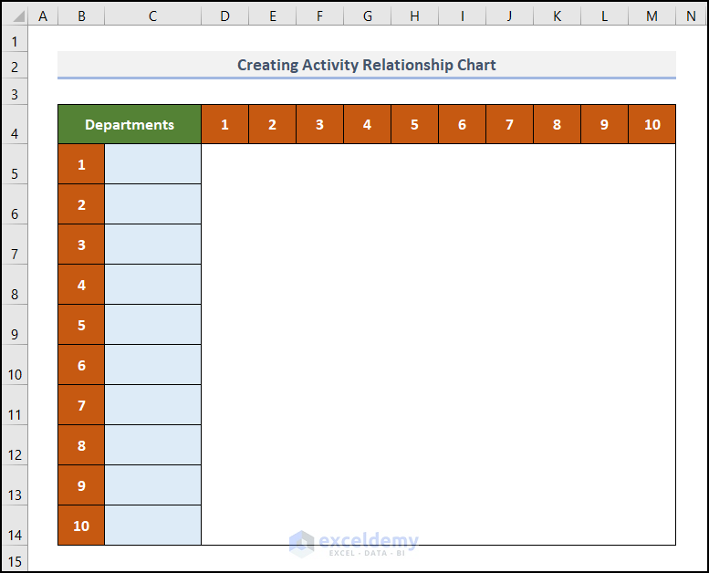
Step 01: Create Basic Outline

In the first and foremost step, we should create a basic outline where all the elements of the chart can accommodate themselves. It’s so simple and easy also. So, let’s see it in action.

📌 Steps:

• At the very beginning, create a table in the B4:M14 range.
• In cell B4, we wrote down the text Departments.
• Besides, we can see 1 to 10 in Column B and in Row 4. These are the serial numbers of the departments which we’ll input in the next step.
• Also, we have left the D5:M14 range blank for future usage.

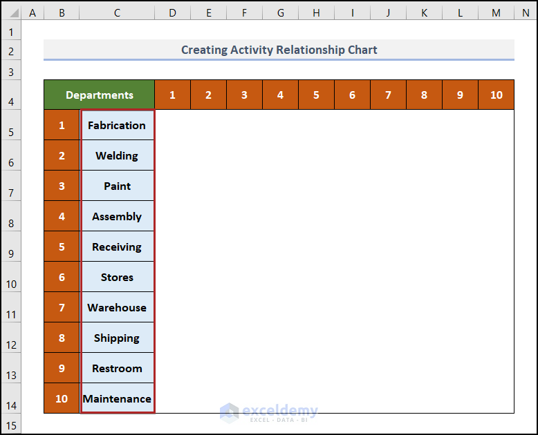
Step 02: Disclosure of Department Names

In the next step, we’ll insert the names of the departments of the facility. Here, we’ll use 10 different departments in our sheet. So, without further delay, let’s dive in!

📌 Steps:

• At this time, write down the name of the departments one after one in the C5:C14 range.
• In this case, we adverted the Fabrication, Welding, Paint, etc. departments.

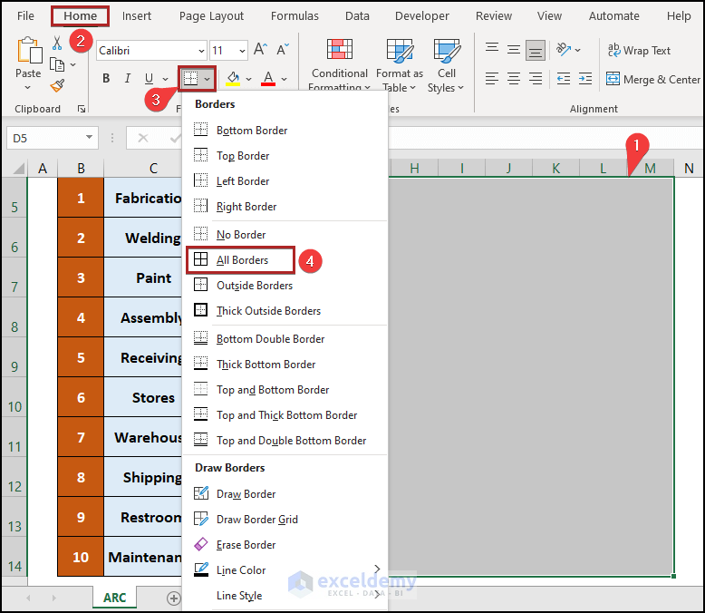
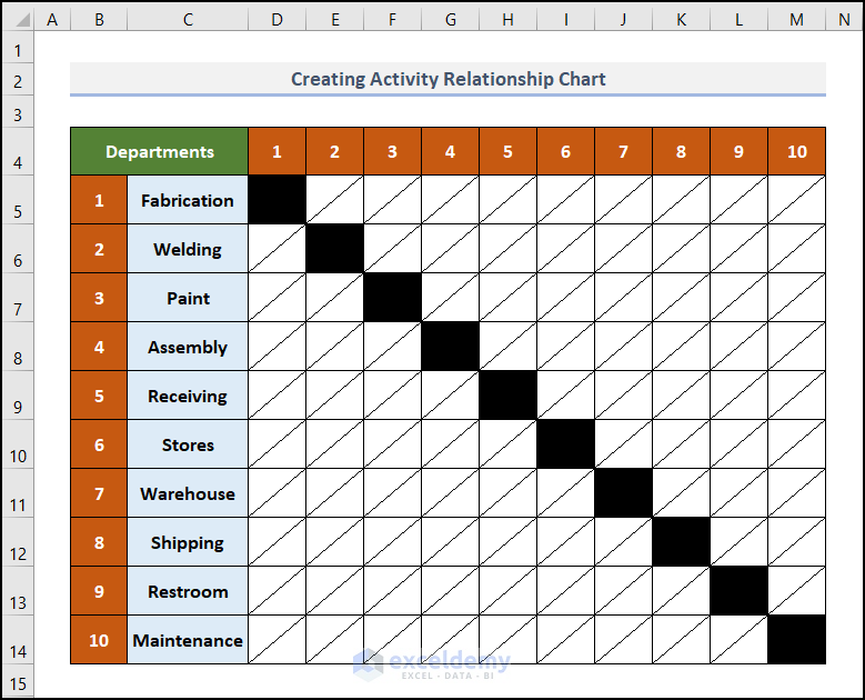
Step 03: Construct Cell Borders

Now, the main part of embellishment comes. We’ll modify the blank spaces in the table to create the Activity Relationship Chart. Let’s see the process in detail.

📌 Steps:

• At first, select cells in the D5:M14 range.
• Then, go to the Home tab.
• After that, click on the Borders drop-down from the Font group of commands.
• Later, select All Borders from the list.

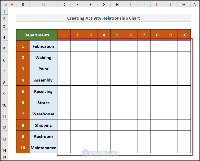
Currently, the worksheet looks like the following image.

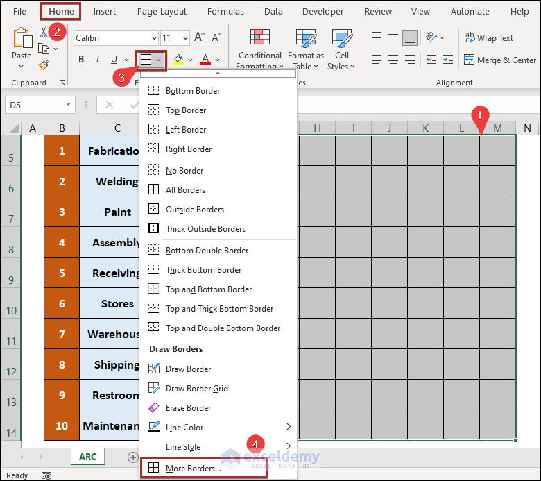
• Again, select the previous range.
• Additionally, repeat the previous steps to open the Borders drop-down list.
• But, this time, select the More Borders option at last.

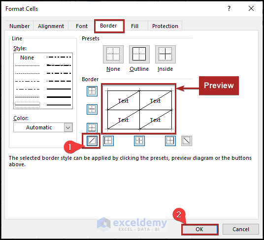
Immediately, the Format Cells dialog box appears before us. Automatically, it will take us to the Border tab.

• Then, apply the diagonal border as shown in the image below.
• As usual, click OK.

Presently, the final result is before our eyes.

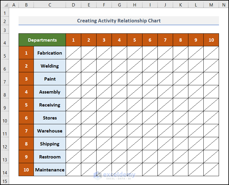
Step 04: Give Closeness Rating and Reasons in Each Cell

In this last step, we’ll do the technical part of this chart. Before starting, the dataset is purely fictitious and used only for your understanding. So, let’s get started.

📌 Steps:

Before inserting the data, we’ll restrict some cells. Because no data will sit in them. To do this,

• Firstly, select the cells along the diagonal in the D5:M14 range.
• Secondly, proceed to the Home tab.
• Thirdly, click on the Fill Color drop-down icon on the Font group.
• Afterward, select Black from the Theme Colors.

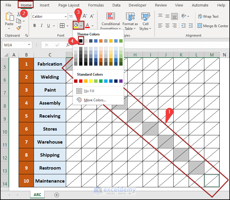
Moreover, the final look is like something below.

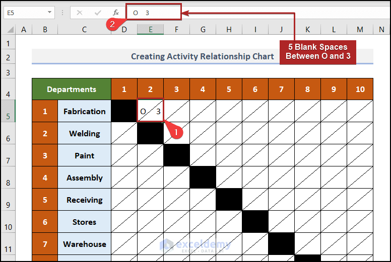
• Now, select cell E5 and write down the following text in that cell.

There are 5 blank spaces between these two letters. We did it intentionally to accommodate these on both sides of the diagonal border in the cell.

• After that, press the ENTER key.

• Similarly, fill up the other cells with correct data.

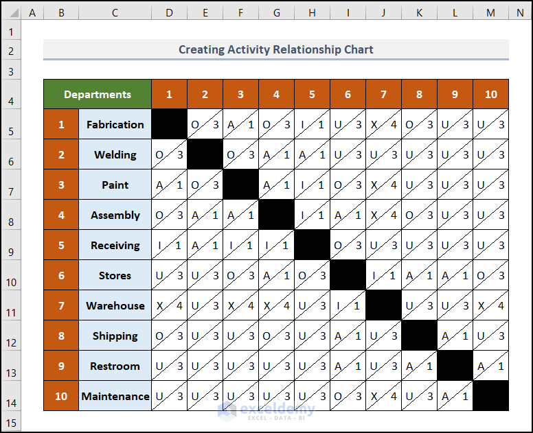
So, If you notice, you’ll see that the data is symmetrical along the corners on both sides of the black cells.
If you want to find the relationship between the Welding and Receiving departments, how could you do that? It’s so easy.
The serial numbers of these two departments are 2 and 5 respectively. So, you will find the result at the intersection of 2 and 5.

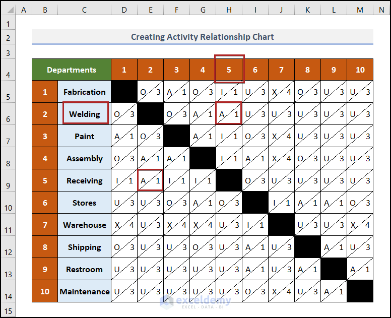
Therefore, 2 and 5 intersect with each other two times. In cells E9 and H6, values are the same. So, the relationship between these two departments is A1. That means their closeness is absolutely necessary, and the flow of material will also happen between them.

Download Practice Workbook

You may download the following Excel workbook for better understanding and practice yourself.

Conclusion

This article explains how to use a continuous probability distribution in Excel in a simple and concise manner. Don’t forget to download the Practice file. Thank you for reading this article. We hope this was helpful. Please let us know in the comment section if you have any queries or suggestions.