When you have a database with case-sensitive values, you might need to match those. Excel has some amazing formulas to match case-sensitive values. The article will describe the possible ways to match case-sensitive values in Excel with suitable examples and proper illustrations.
How to Find Case Sensitive Match in Excel: 7 Ways
Assuming that we have the following sample dataset which we are going to use in the next sections.
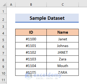
You can see that there are two columns containing ID and Name of people working in a company. In addition, notice that the database contains some case-sensitive values as well. Now, we will demonstrate how to match case-sensitive values in Excel through 7 different formulas.
1. Using EXACT Function
The shortest formula uses the the EXACT function. This function matches cells with exactness. It takes two texts to compare and give the result as Boolean True or False.
Let’s say we want to match values in the cell C8 and cell C10 of the dataset.
The formula for the given dataset will be:
=EXACT(C8,C10)
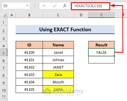
The result shows FALSE though the value matches due to the difference in the case.
You can also check for other values. Let’s say we want to compare the cells, C5 and C7.
The formula will look like:
=EXACT(C5,C7)
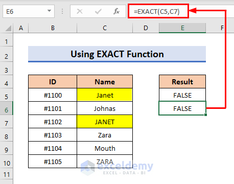
Due to case-sensitive issues, the result will also be false for this one. Observe the result below.
2. Applying Nested OR and EXACT Functions
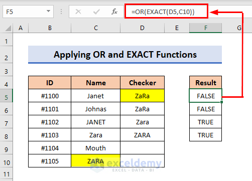
Furthermore, you can use nested OR and EXACT formulas to match values in a range.
Here, we have created a new column for checker values. Then compare the values in this new column with values in the dataset.
The formula for this will be:
=OR(EXACT(D5,C10))
or,
=OR(EXACT(D6,C8))
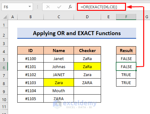
Notice: The checker value does not match with any of the values in the range and so shows FALSE.
Now if we change the checker value with exact cases you can observe that the result shows TRUE. The results are shown below.
🔎 Formula Explanation
The TEXT function takes two texts to compare and gives the result as Boolean True or False.
And the OR function takes the logic from where any of the logic needs to be fulfilled to get a result as Boolean TRUE. Unless it shows Boolean False.
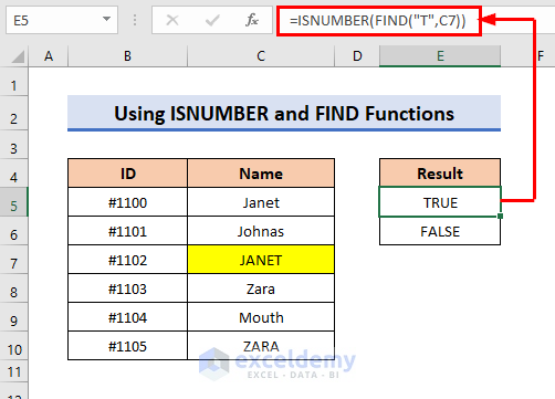
3. Using ISNUMBER with FIND and IF Functions
You can use the nested ISNUMBER and FIND formula to match whether a cell value contains a particular character or not. The FIND function returns the starting position of one text string with another text string. It is case-sensitive by nature. And the ISNUMBER function returns whether a value is a number and returns TRUE or FALSE.
Let’s check for T and j in dataset cell C7.
The formula is:
=ISNUMBER(FIND("T",C7))
or
=ISNUMBER(FIND("j",C7))
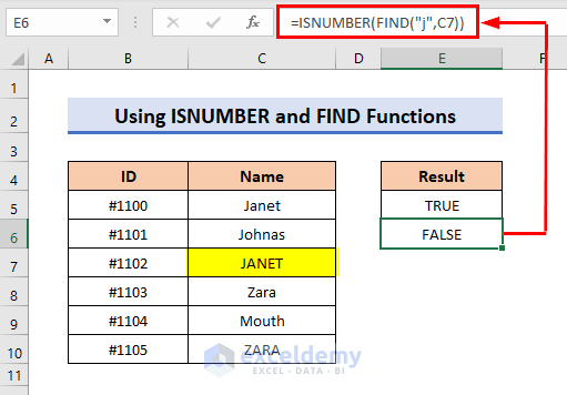
The result shows TRUE and FALSE respectively.
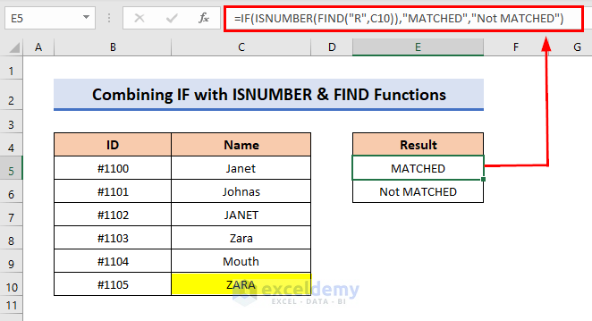
4. Combining IF with ISNUMBER and FIND Functions
You can add the IF function with the formula stated in Method 3 if you want to get result as a remark instead of Boolean ones.
Now, let’s check for R and a in Dataset cell C10.
Then, the formula becomes,
=IF(ISNUMBER(FIND("R",C10)),"MATCHED","Not MATCHED")
or
=IF(ISNUMBER(FIND("a",C10)),"MATCHED","Not MATCHED")
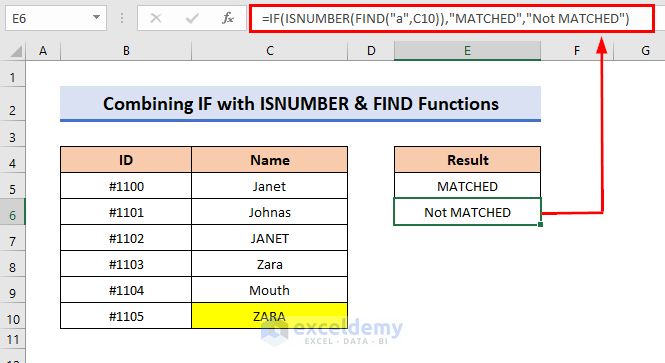
The result is perfectly working as you can observe in the above pictures.
🔎 Formula Explanation
The FIND function returns the starting position of one text string with another text string. It is case-sensitive by nature. And ISNUMBER function returns whether a value is a number and returns TRUE or FALSE.
Finally, the IF function checks whether the condition is met and returns MATCHED, else it returns Not MATCHED.
5. Using Nested SUMPRODUCT and EXACT Functions
We can combine The SUMPRODUCT and EXACT functions to create a nested formula to match case-sensitive values. Nevertheless, it is worth mentioning that the SUMPRODUCT function can only return numbers and not text.
Let us modify our dataset to have only numbers in the ID column.
The formula for this will be:
=SUMPRODUCT(--EXACT(C7,C5:C10),B5:B10)
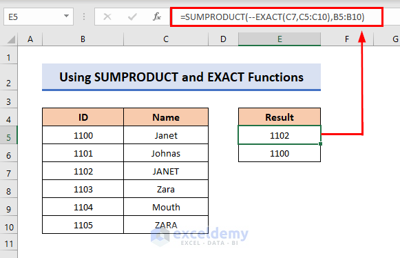
🔎 Formula Explanation
The EXACT function takes two texts to compare and gives the result as Boolean True or False.
EXACT(C7,C5:C10) returns => {FALSE;FALSE;TRUE;FALSE;FALSE;FALSE}
The SUMPRODUCT function takes arrays to give the arithmetic sum of the corresponding arrays.
SUMPRODUCT(–EXACT(C7,C5:C10),B5:B10) = SUMPRODUCT(–{FALSE;FALSE;TRUE;FALSE;FALSE;FALSE},{1100;1101;1102;1103;1104;1105}) = 1102
So, Final Output => 1102
or,
=SUMPRODUCT(--EXACT(C5,C5:C10),B5:B10)
for getting results for cells C7 and C5 in the dataset.
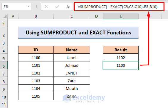
You can see the result shows for JANET and Janet correctly. Hence, it works for case-sensitive values.
6. Applying INDEX and MATCH Functions
Apart from these, the formula with nested INDEX and MATCH functions can be used to match case-sensitive values in Excel. This will return the value if matched exactly.
Let us check for “JANET” and “Zara” from the dataset.
The formula is:
=INDEX(C5:C10, MATCH(TRUE, INDEX(EXACT(C7, C5:C10), ), 0))
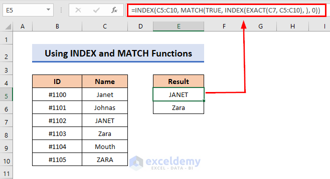
🔎 Formula Explanation
EXACT(C7, C5:C10) returns => {FALSE;FALSE;TRUE;FALSE;FALSE;FALSE}
INDEX(EXACT(C7, C5:C10), ) returns => {FALSE;FALSE;TRUE;FALSE;FALSE;FALSE}
MATCH(TRUE, INDEX(EXACT(C7, C5:C10), ), 0) returns => MATCH(TRUE,{FALSE;FALSE;TRUE;FALSE;FALSE;FALSE}) => 3
INDEX(C5:C10, MATCH(TRUE, INDEX(EXACT(C7, C5:C10), ), 0)) = INDEX(C5:C10, 3) = JANET
So, Final Output => JANET
Similarly,
=INDEX(C5:C10, MATCH(TRUE, INDEX(EXACT(C8, C5:C10), ), 0))
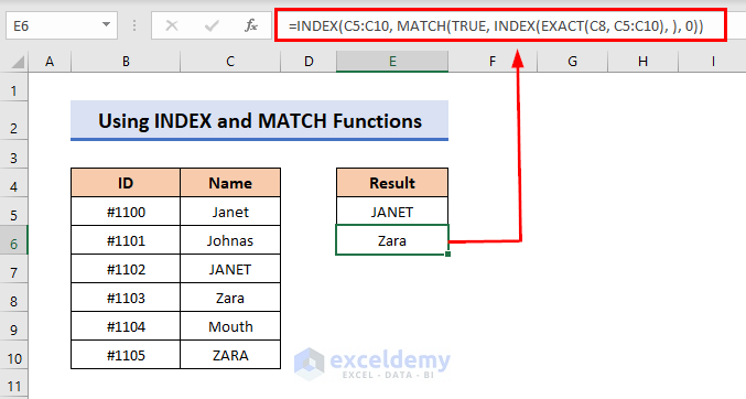
The result finds the exact match for both the values and so provides the values in return.
7. Utilizing LOOKUP Function
Last but not least, the LOOKUP function also works to match values. But those do not work for case-sensitive issues. However, the LOOKUP function can be nested with EXACT and IF functions to get results for the match of case-sensitive values. There are mainly two types of LOOKUP functions that worked fine in this case. Those are VLOOKUP and HLOOKUP functions. We will learn how to use them in this case from below.
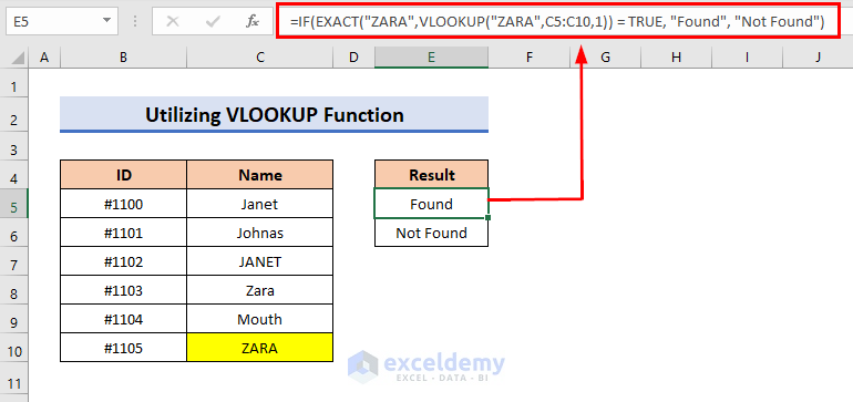
7.1. Using VLOOKUP Function
Let’s consider the value ZARA to match using the VLOOKUP function.
The formula will be:
=IF(EXACT("ZARA",VLOOKUP("ZARA",C5:C10,1)) = TRUE, "Found", "Not Found")
🔎 Formula Explanation
The VLOOKUP function looks for a value in the leftmost column of a table and then returns a value in the same row from a column you specify. By default, the table must be in ascending order.
VLOOKUP(“ZARA”,C5:C10,1)) returns => “ZARA”
EXACT(“ZARA”,VLOOKUP(“ZARA”,C5:C10,1)) = TRUE becomes EXACT(“ZARA”,”ZARA”) = TRUE and returns => TRUE
Finally, IF(EXACT(“ZARA”,VLOOKUP(“ZARA”,C5:C10,1)) becomes TRUE, “Found”, “Not Found”)IF(TRUE, “Found”, “Not Found”) and returns => Found
So, the result shows “Found” since the value is matched in the range of data.
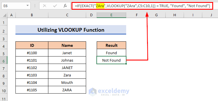
Now, if we change the case form in the value the result will show “Not Found”. The result is shown below.
7.2. Using HLOOKUP Function
Subsequently, the HLOOKUP function can also be used for the purpose in a similar manner. Both VLOOKUP and HLOOKUP work similarly. The only difference is that VLOOKUP looks up in columns and HLOOKUP in rows. Thus, the letters H and V stand for Horizontal and Vertical respectively.
The formula for suppose Janet :
=IF(EXACT("Janet",HLOOKUP("Janet",C5:C10,1)) = TRUE, "Found", "Not Found")
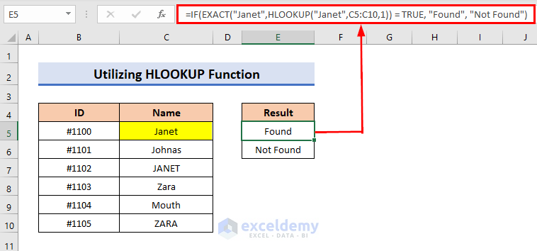
The result works perfectly.
Again, if we change the case form of the text the result will be the opposite. See the picture below for matching JaNet
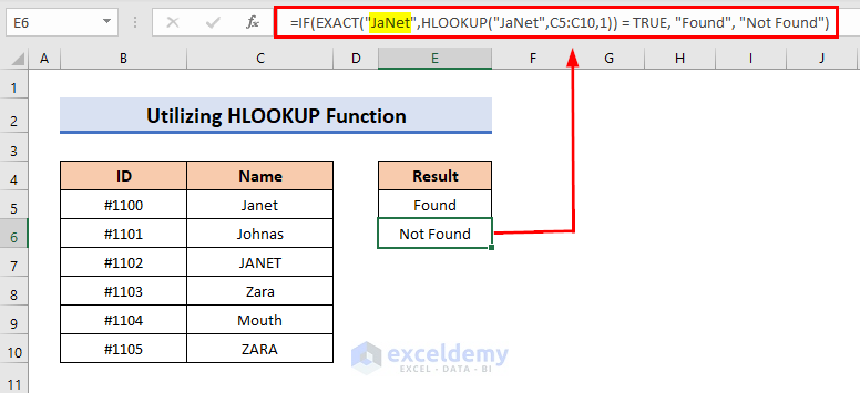
You won’t find the result as the case doesn’t match.
Download Practice Workbook
For practice, you can download the workbook from the link below.
Conclusion
The article demonstrated 6 amazing formulas to match case-sensitive values in Excel. The formulas use functions like EXACT, IF, SUMPRODUCT, VLOOKUP, and so on. Hopefully, the article was helpful to you. Anyway, if you have any queries you can ask in the comment section.
<< Go Back to | Excel Match | Learn Excel
Get FREE Advanced Excel Exercises with Solutions!
