In MS Excel, the VLOOKUP function is the most important function to search for any data from a dataset or table. For calculation, sometimes we may need to get the summation of some searched data. In this way, there is a possible solution in Excel. However, we could simply use Excel’s VLOOKUP and SUM functions to get the summation from multiple rows. In this article, we will see 4 different examples of how we can use VLOOKUP to Sum multiple rows in Excel.
Use VLOOKUP to Sum Multiple Rows in Excel: 4 Ideal Examples
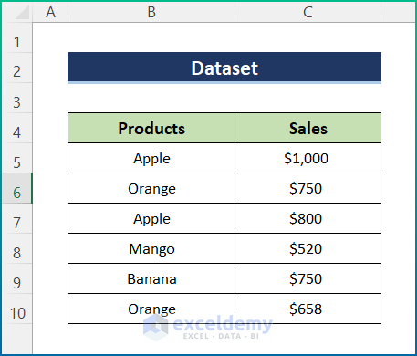
In this tutorial, we will show you how to use VLOOKUP and SUM functions in multiple rows in Excel. Here, we have used 4 different examples to make you understand the scenario properly. For the purpose of demonstration, we have used the following sample dataset.
1. VLOOKUP and Sum Matched Values in Multiple Rows
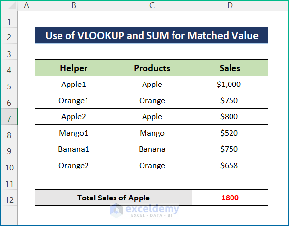
In our first method, we’ll create a Helper Column using the COUNTIF function to find exact matches with VLOOKUP in Excel. However, it becomes difficult to utilize the process if you have a long dataset containing a large amount of data. Here, we’ll find the product Apple using VLOOKUP and the sum of the total sales of Apple in this example. Hence, follow the steps below.
📌 Steps:
- First, write the following formula in cell B5 to create the Helper Column.
=C5&COUNTIF($C$5:$C5,C5)
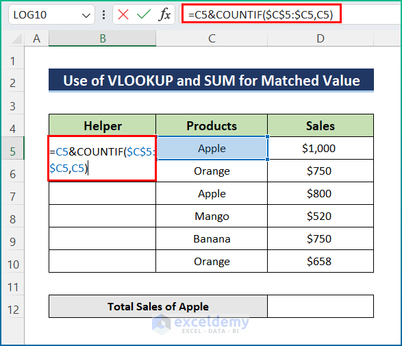
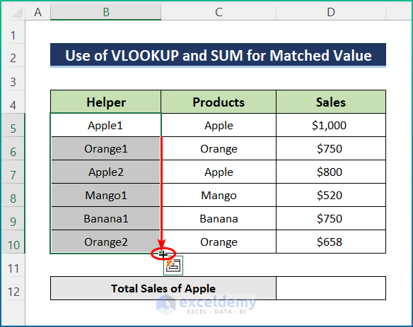
- Then, click Enter and use the AutoFill tool to the whole column.
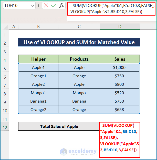
- After that, select cell D12 and write the following formula.
=SUM(VLOOKUP("Apple"&1,B5:D10,3,FALSE),VLOOKUP("Apple"&2,B5:D10,3,FALSE))
🔎 Formula Breakdown:
- Firstly, using the VLOOKUP function, the criteria: Apple is matched with ranges B5:D10 from the dataset.
- Here, you have to search twice, as the Helper column shows Apple twice.
- After that, the VLOOKUP function extracts the values of the matched cells.
- Lastly, the SUM function provides the sum of the output values provided by the VLOOKUP function.
- Last, hit the Enter button in order to get the total sales of Apple.
Read More: How to Use VLOOKUP for Rows in Excel
2. Insert SUMPRODUCT Function to VLOOKUP and Sum
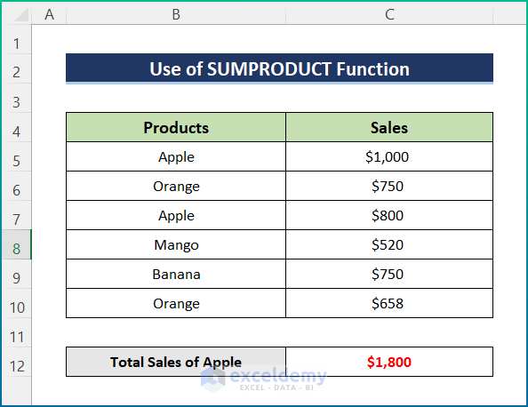
The SUMPRODUCT function is one of the most fantastic functions in Excel. Fortunately, it can work with multiple arrays and return the sum of the values maintaining the criteria. However, SUMPRODUCT takes one or more arrays as an argument, multiplies the corresponding values of all the arrays, and then returns the sum of the products. In this case, we will find out the total sales of Apples directly.
📌 Steps:
- In the beginning, select cell C12 and insert the following formula.
=SUMPRODUCT((B5:B10="Apple")*C5:C10)
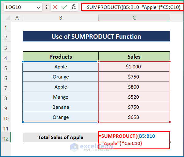
- In the end, press Enter to get a similar output.
Read More: How to VLOOKUP and SUM Across Multiple Sheets in Excel
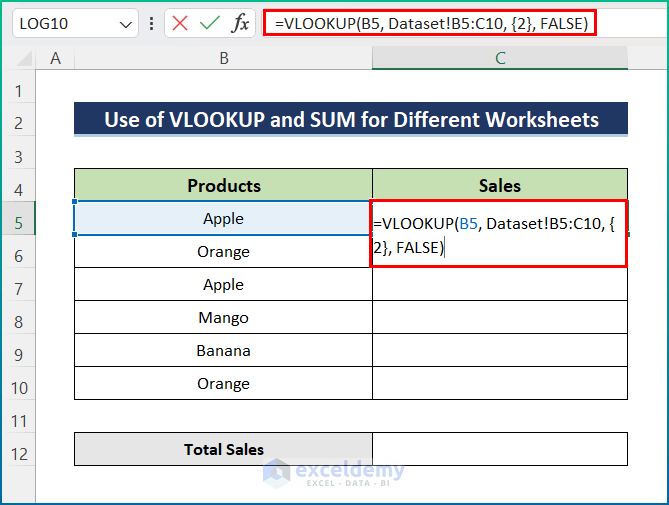
3. VLOOKUP and Sum Multiple Rows from Different Worksheets
Furthermore, let’s assume the above scenario in different worksheets. For example, we want to extract the data of sales from the Dataset sheet by using the VLOOKUP function and calculate the Total Sales of all products using the SUM function.
📌 Steps:
- Firstly, click on cell C5 and insert the formula below.
=VLOOKUP(B5, Dataset!B5:C10, {2}, FALSE)
Note:
In the formula, {2} indicates the column index number. It starts from 1 which indicates the first column in an Excel sheet. Here, our dataset starts from the second column and that’s why we have used 2 as column index.
- Secondly, apply the AutoFill tool to the entire column of the dataset.
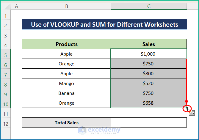
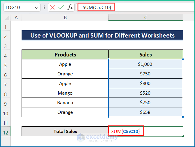
- Thirdly, select cell C12.
- Fourthly, enter the following formula.
=SUM(C5:C10)
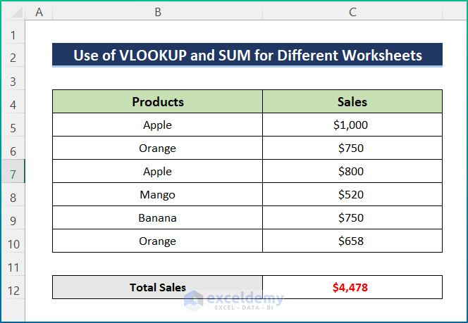
- Finally, press the Enter button to get the result.
Read More: How to Combine SUMIF and VLOOKUP in Excel
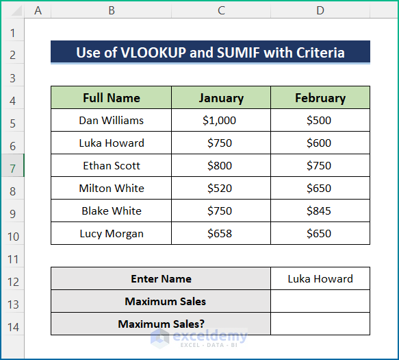
4. VLOOKUP and SUMIF Multiple Rows with Criteria
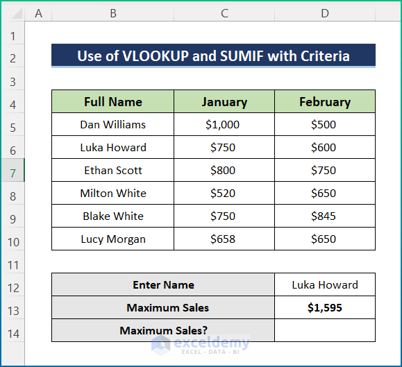
Last but not least, we will combine the VLOOKUP and SUMIF functions in multiple rows with specific criteria. In this section, we will find out the total maximum sales from the dataset. However, we will match if the searched Name has the Maximum Sales or not. If yes, then it prints “Yes”; otherwise “No”. For the purpose of demonstration, we have chosen the following sample dataset.
📌 Steps:
- Initially, select cell D13 and write down the formula below.
=MAX(SUM(C5:D5),SUM(C6:D6),SUM(C7:D7),SUM(C8:D8),SUM(C9:D9),SUM(C10:D10))
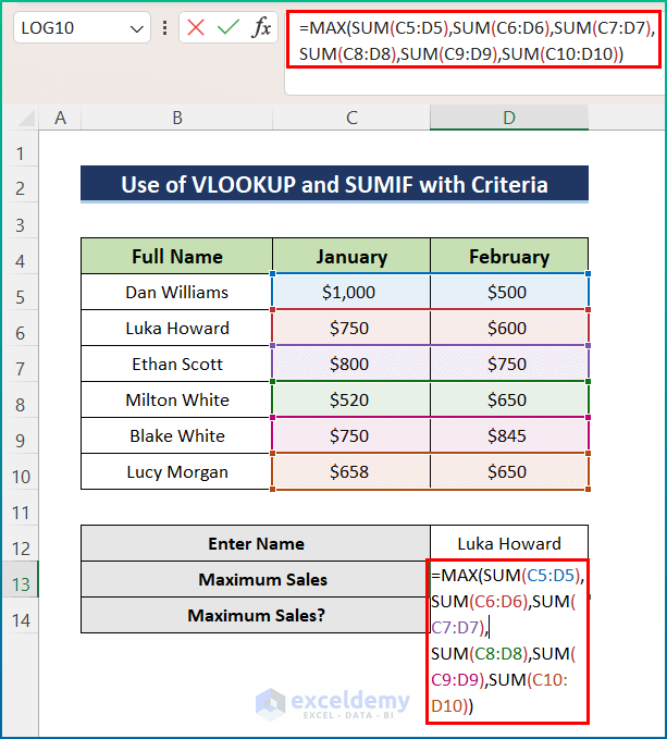
- Next, press the Enter button to find the Maximum Sales.
- After that, insert the formula below in cell D14.
=IF(SUM(VLOOKUP(D12, $B$5:$D$10,{2,3}, FALSE))>=D13,"Yes","No")
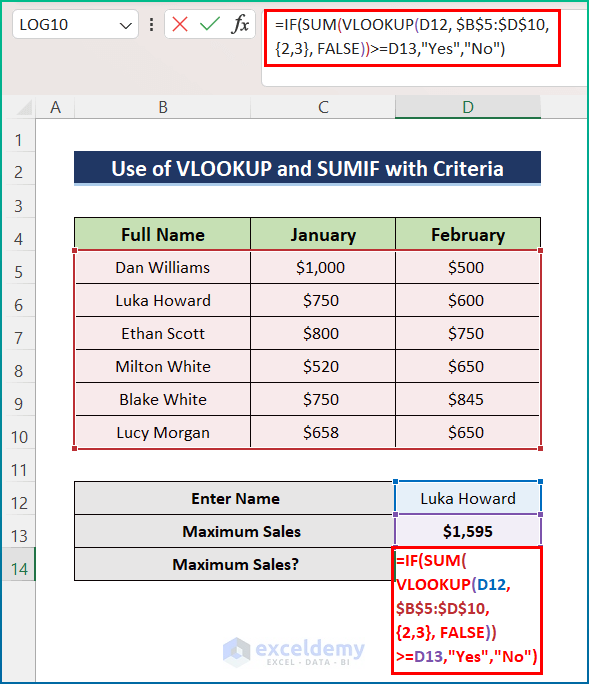
🔎 Formula Breakdown:
- Firstly, in the IF function, SUM(VLOOKUP(D12, $B$5:$D$10, {2,3}, FALSE))>=D13 is the logical condition.
- Secondly, {2,3} is an argument of the VLOOKUP function which indicates the column index number. Usually, it starts from 1 which indicates the first column in an Excel sheet.
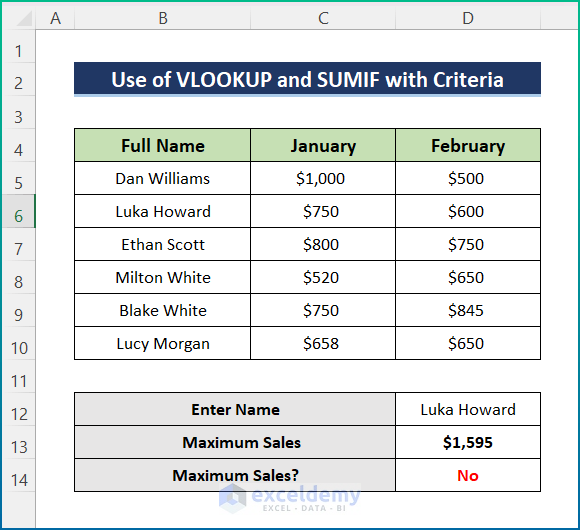
- However, the VLOOKUP function checks if the entered Name’s total sales are greater than or equal to our predefined maximum sales or not. Here, it searched for Luka Howard and provided the amount of sales for January and February.
- After that, the SUM function provides the sum of the sales amount received from the VLOOKUP function. However, the output is 1350$.
- Finally, the IF function checks the condition. Here, the maximum sale is given as 1595$ and the formula will check whether the output we received is maximum or not. If the sales match then it will print “Yes” otherwise “No”.
- Lastly, hit the Enter key to get the final result.
Read More: INDEX MATCH vs VLOOKUP Function
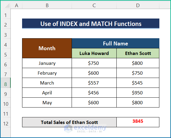
How to Sum Multiple Rows with INDEX and MATCH Functions
However, we can combine the INDEX and MATCH functions in order to find the sum for multiple rows. However, this alternative process is much easier to operate. Here, we will calculate the total sales of employee Ethan Scott for various months of the year. For the purpose of demonstration, I have changed the previous dataset. Hence, go through the steps below in order to complete the operation properly.
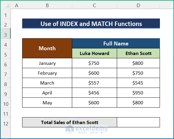
📌 Steps:
- Firstly, insert the following formula in cell D12.
=SUM(INDEX(C5:D10,,MATCH("Ethan Scott",C5:D5,0)))
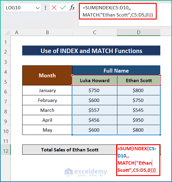
- Afterward, press Enter in order to calculate the total sales of Ethan Scott.
Things to Remember
- Firstly, if the searched value is not present in the given dataset, then all these functions will return this #NA Error.
- Similarly, if col_index_num is greater than the number of columns in table-array, you’ll get the #REF! Error value.
- Finally, you’ll get the #VALUE! Error value If the table_array is less than 1.
Download Practice Workbook
You can download the workbook used for the demonstration from the download link below.
Conclusion
These are all the steps you can follow to operate VLOOKUP SUM across multiple rows in Excel. Overall, in terms of working with time, we need this for various purposes. I have shown multiple methods with their respective examples, but there can be many other iterations depending on numerous situations. Hopefully, you can now easily create the needed adjustments. I sincerely hope you learned something and enjoyed this guide. Please let us know in the comments section below if you have any queries or recommendations.
Further Readings
- Combining SUMPRODUCT and VLOOKUP Functions in Excel
- How to Use VLOOKUP with COUNTIF
- Excel LOOKUP vs VLOOKUP
- XLOOKUP vs VLOOKUP in Excel
- How to Use Nested VLOOKUP in Excel
- IF and VLOOKUP Nested Function in Excel
- How to Use IF ISNA Function with VLOOKUP in Excel
- How to Use VLOOKUP Function with INDIRECT Function in Excel
- How to Use IFERROR with VLOOKUP in Excel
- VLOOKUP with IF Condition in Excel
<< Go Back to Excel VLOOKUP Sum | Excel VLOOKUP Function | Excel Functions | Learn Excel
Get FREE Advanced Excel Exercises with Solutions!

JazzakAllahKhair Brother.
Hey, man. It looks like you are getting the sum of the columns (not the rows as indicated) in the first example.
what {2,3} mean?
Hello QUAN,
Thanks for your question. Here, {2,3} defines the cell number of the defined range B5:D10. 2 defines the row number and 3 defines the column number. Setting B5 as the base point and moving two rows and three columns, we will have the D6 cell which is expressed here with {2,3}.