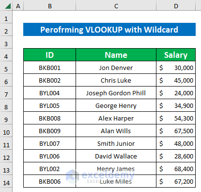
The dataset showcases ID, Name and Salary.
To find the salary of a specific sales representative:
Method 1 – Using the VLOOKUP Function with a Single Wildcard in Excel
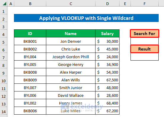
1.1. Searching for Starting Words or Characters
Find Harper’s salary:
Steps:
- In F7, enter the following formula:
=VLOOKUP("*"&F5&"*",C5:D14,2,FALSE)
- F5 is the lookup value. The Asterisk ( * ) joins the text in the named range with a wildcard. The ampersand (&) is used to concatenate.
- The Lookup_Array is C5:D14
- The Col_index_num is 2
- For an EXACT match, FALSE is used.
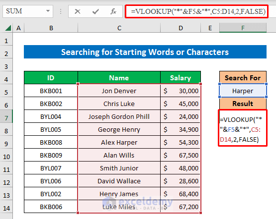
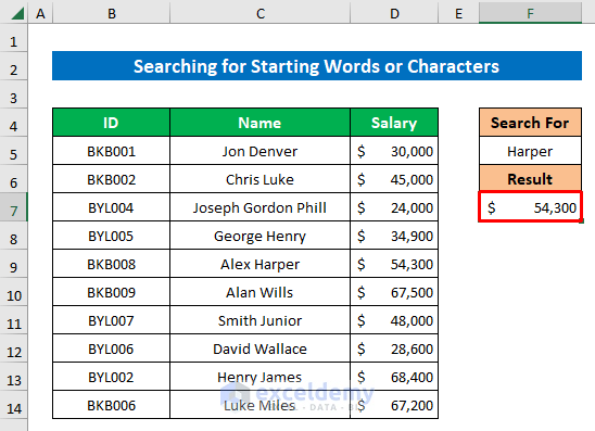
- Press ENTER.
Alex Harper’s salary is displayed.
Read More: How to Use VLOOKUP to Find Partial Text from a Single Cell
1.2. Finding End Words or Characters
Steps:
- In F7, enter the following formula:
=VLOOKUP(F5&"*",C5:D14,2,FALSE)
Where,
The lookup value is F5&”*”. The asterisk sign ( * ) is used to find the ending words and the ampersand ( & ) is used to concatenate them.
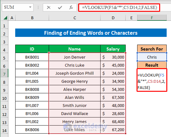
- Press ENTER.
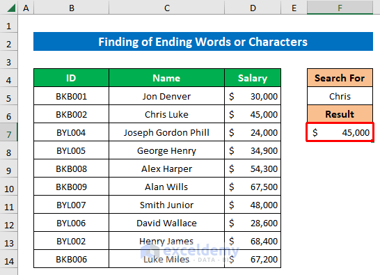
This is the output.
1.3. Identifying a Cell Containing a Specific Letter
To get the salary for the ID: “BKB002”:
Steps:
- In F7, enter the following formula:
=VLOOKUP("?KB002",B5:D14,3,FALSE)
The lookup_value is ?KB002. The question mark (?) is used as a wildcard to return the exact value.
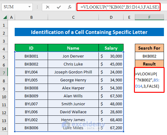
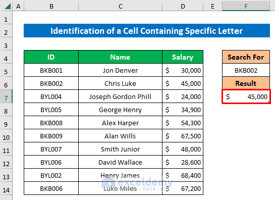
- Press ENTER.
Method 2 – Applying the VLOOKUP with Multiple Wildcards in Excel
2.1. Finding Cells Containing Multiple Letters with Wildcards
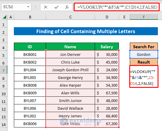
To see the salary of a salesperson whose middle name is Gordon:
Steps:
- In F7, enter the following formula:
=VLOOKUP("*"&F5&"*",C5:D14,2,FALSE)
“*”&F5&”*” is the lookup value. The asterisk and the ampersand sign on both sides of the cell reference are used to match missing words on both sides.
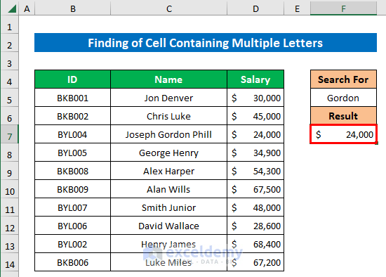
- Press ENTER.
This is the output.
Read More: How to Use Excel VLOOKUP to Find the Closest Match
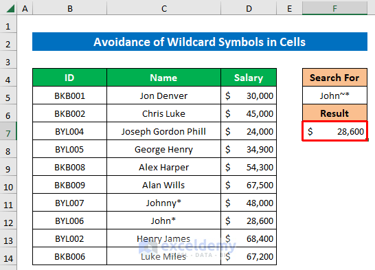
2.2. Considering Cells with Wildcard Symbols
To find the salary of: John*.
Step 1:
- In F7, enter the following formula:
=VLOOKUP(F5,C5:D14,2,FALSE)
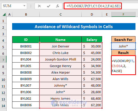
- Press ENTER.

The function took the asterisk as a wildcard and returned the value.
Step 2:
To avoid the wildcard:
- In F7, enter the following formula:
=VLOOKUP(F5&"*~",C5:D14,2,FALSE)
The lookup value is F5&”*~”. The tilde (~) will nullify the effect of the asterisk and the function will return the exact value.
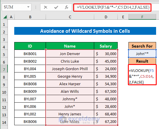
- Press ENTER.
Method 3 – Using the VLOOKUP with a Wildcard to Find a Partial Match in Excel
Steps:
- In F7, enter the following formula:
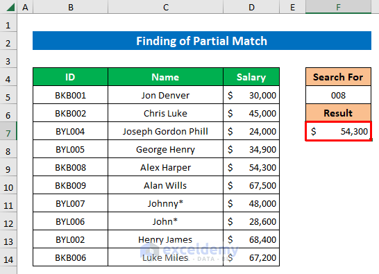
=VLOOKUP("???"&F5,B5:D14,3,0)
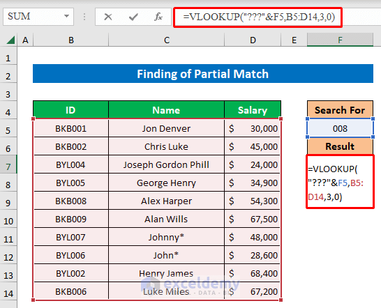
- Press ENTER.
This is the output.
Read More: Use VLOOKUP to Find Multiple Values with Partial Match in Excel
Things to Remember
- The Asterisk (*) can match any number of characters, whereas the question mark (?) matches one character only.
- The VLOOKUP function always searches the lookup values from the leftmost top column to the right.
Download Practice Workbook
Download the practice worksheet.
Related Articles
- How to Use VLOOKUP to Find Approximate Match for Text in Excel
- How to Vlookup Partial Match for First 5 Characters in Excel
- Excel VLOOKUP for Partial Match in Table Array
<< Go Back to VLOOKUP Partial Match | Excel VLOOKUP Function | Excel Functions | Learn Excel
Get FREE Advanced Excel Exercises with Solutions!
