Introduction to VLOOKUP Function
The VLOOKUP function looks for a value in the left-most column of a table array and then returns a value in the same row from a column to the right with the offset you specify.
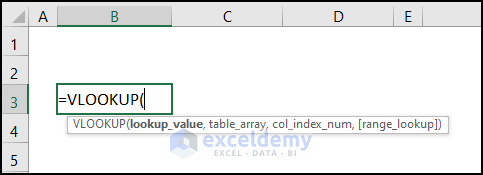
- Syntax:
=VLOOKUP(lookup_value,table_array,col_index_num,[range_lookup])
- Argument Explanation:
| Argument | Required/Optional | Explanation |
|---|---|---|
| lookup_value | Required | the value we want to lookup |
| table_array | Required | range of cells containing input data |
| col_index_num | Required | column number of the lookup value |
| range_lookup | Optional | TRUE refers to an approximate match, FALSE indicates an exact match |
- Return Parameter:
Returns an exact or approximate value corresponding to the user’s input value.
Using VLOOKUP Function to Return the Highest Value in Excel: 4 Simple Ways
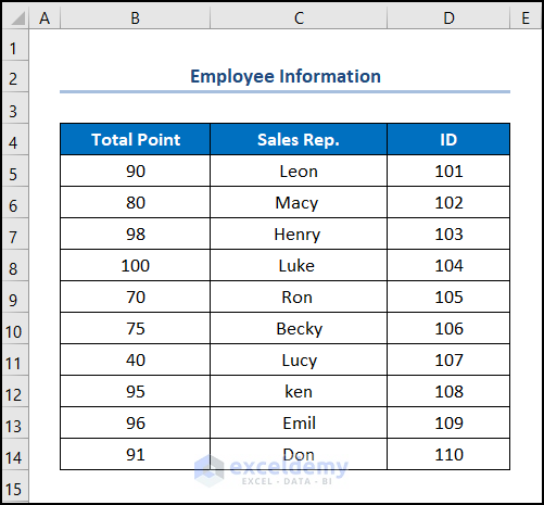
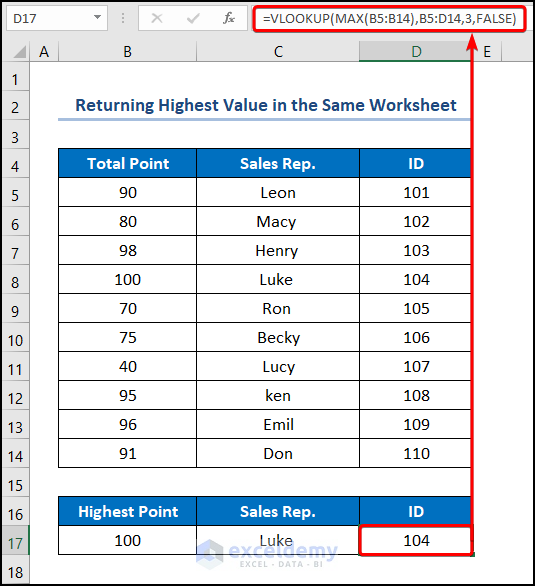
Let’s consider the Employee Information dataset shown in the B4:D14 cells, which shows the Total Point, Sales Rep, and ID of the employees. We want to return the highest value with the VLOOKUP function in Excel.
Method 1 – Return Highest Value in the Same Worksheet
Steps:
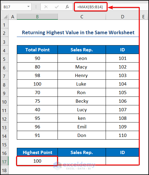
- Go to the B17 cell and enter the formula given below:
=MAX(B5:B14)
Here, the B5:B14 cells refer to the “Total Point” column.
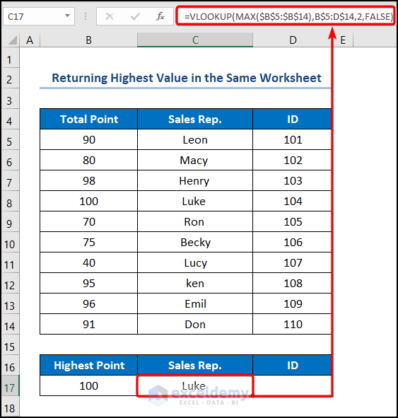
- Move to the C17 cell and type in the expression below.
=VLOOKUP(MAX($B$5:$B$14),B$5:D$14,2,FALSE)
Formula Breakdown:
- MAX($B$5:$B$14) → returns the largest value in a set of values. Here, the $B$5:$B$14 cells is the number1 argument which represents the “Total Point” column.
- Output → 99
- VLOOKUP(MAX($B$5:$B$14),B$5:D$14,2,FALSE) → looks for a value in the left-most column of a table, and then returns a value in the same row from a column you specify. Here, MAX($B$5:$B$14) ( lookup_value argument) is mapped from the B$5:D$14 (table_array argument) array. Next, 2 (col_index_num argument) represents the column number of the lookup value. Lastly, FALSE (range_lookup argument) refers to the Exact match of the lookup value.
- Output → Luke
- Navigate to the D17 cell and insert the following formula:
=VLOOKUP(MAX(B5:B14),B5:D14,3,FALSE)
For instance, the B4:B14 cells point to the “Total Point” column.
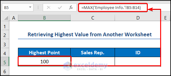
Method 2 – Retrieve Highest Value from Another Worksheet
Steps:
- Enter the formula given below into cell B5:
=MAX('Employee Info.'!B5:B14)
In this case, “Employee Info.” is the name of the worksheet whereas the B5:B14 cells represent the dataset.
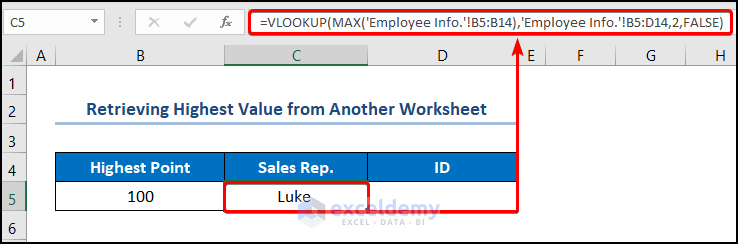
- Move to the adjacent C5 cell and enter the following:
=VLOOKUP(MAX('Employee Info.'!B5:B14),'Employee Info.'!B5:D14,2,FALSE)
In this scenario, the B5:B14 cells represent the dataset, and the “Employee Info.” is the name of the worksheet.
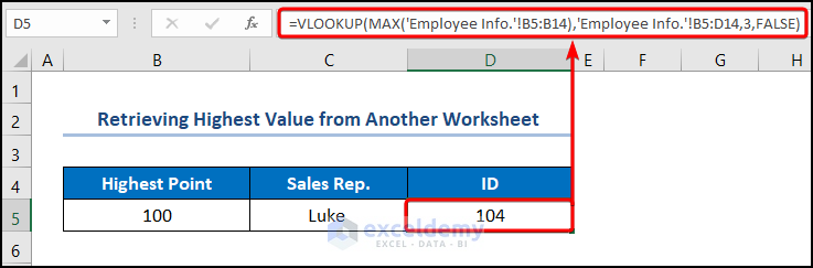
- Input a similar formula into D5.
=VLOOKUP(MAX('Employee Info.'!B5:B14),'Employee Info.'!B5:D14,3,FALSE)
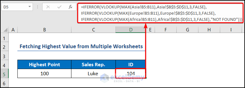
Method 3 – Fetch Highest Value from Multiple Worksheets
Let’s assume the Employee Information for Asia Region dataset which displays the Total Point, Sales Rep, and ID respectively.

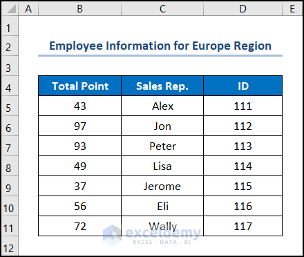
Similarly, we have the Employee Information for Europe Region dataset.
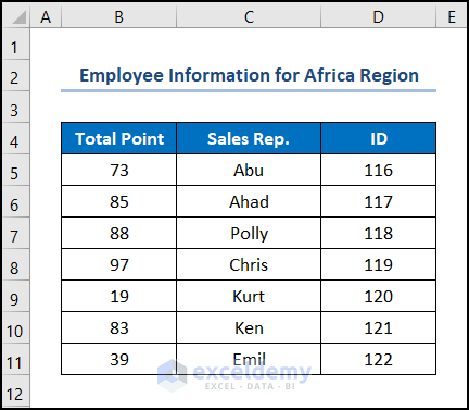
Lastly, the dataset of Employee Information for Africa Region is available.
Steps:
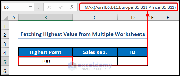
- Navigate to the B5 cell of the result worksheet and insert the following expression into the Formula Bar:
=MAX(Asia!B5:B11,Europe!B5:B11,Africa!B5:B11)
Here, the B5:B11 cells indicate the “Total Point” column in the “Asia”, “Europe”, and “Africa” worksheets.
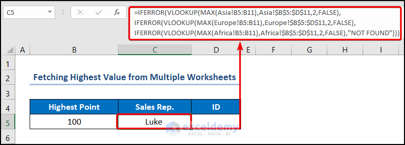
- Enter the expression below into the C5 cell:
=IFERROR(VLOOKUP(MAX(Asia!B5:B11),Asia!$B$5:$D$11,2,FALSE),IFERROR(VLOOKUP(MAX(Europe!B5:B11),Europe!$B$5:$D$11,2,FALSE),IFERROR(VLOOKUP(MAX(Africa!B5:B11),Africa!$B$5:$D$11,2,FALSE),"NOT FOUND")))
Formula Breakdown:
- VLOOKUP(MAX(Asia!B5:B11),Asia!$B$5:$D$11,2,FALSE) → here, MAX(Asia!B5:B11) ( lookup_value argument) is mapped from the Asia!$B$5:$D$11(table_array argument) array in the “Asia” worksheet. Next, 2 (col_index_num argument) represents the column number of the lookup value. Lastly, FALSE (range_lookup argument) refers to the Exact match of the lookup value.
- Output → Luke
- VLOOKUP(MAX(Europe!B5:B11),Europe!$B$5:$D$11,2,FALSE) → the MAX(Europe!B5:B11) ( lookup_value argument) is mapped from the Europe!$B$5:$D$11(table_array argument) array in the “Europe” worksheet.
- Output → Jon
- VLOOKUP(MAX(Africa!B5:B11),Africa!$B$5:$D$11,2,FALSE) → here, MAX(Africa!B5:B11) ( lookup_value argument) is mapped from the Africa!$B$5:$D$11(table_array argument) array in the “Africa” worksheet.
- Output → Chris
- IFERROR(VLOOKUP(MAX(Asia!B5:B11),Asia!$B$5:$D$11,2,FALSE),IFERROR(VLOOKUP(MAX(Europe!B5:B11),Europe!$B$5:$D$11,2,FALSE),IFERROR(VLOOKUP(MAX(Africa!B5:B11),Africa!$B$5:$D$11,2,FALSE),”NOT FOUND”))) → becomes
- IFERROR((“Luke”, “Jon”, “Chris”),”NOT FOUND”) →The IFERROR function returns value_if_error if the error has an error and the value of the expression itself otherwise. Here, the (“Luke”, “Jon”, “Chris”) is the value argument, and “NOT FOUND” is the value_if_error argument. In this case, the function returns the name corresponding to the “Highest Point”.
- Output → Luke
- Copy and paste the following formula into the D5 cell to get the employee ID.
=IFERROR(VLOOKUP(MAX(Asia!B5:B11),Asia!$B$5:$D$11,3,FALSE),IFERROR(VLOOKUP(MAX(Europe!B5:B11),Europe!$B$5:$D$11,3,FALSE),IFERROR(VLOOKUP(MAX(Africa!B5:B11),Africa!$B$5:$D$11,3,FALSE),"NOT FOUND")))
Read More: VLOOKUP with Numbers in Excel
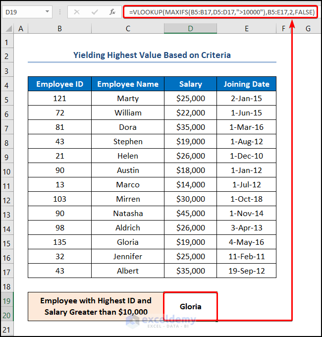
Method 4 – Yield Highest Value Based on Criteria
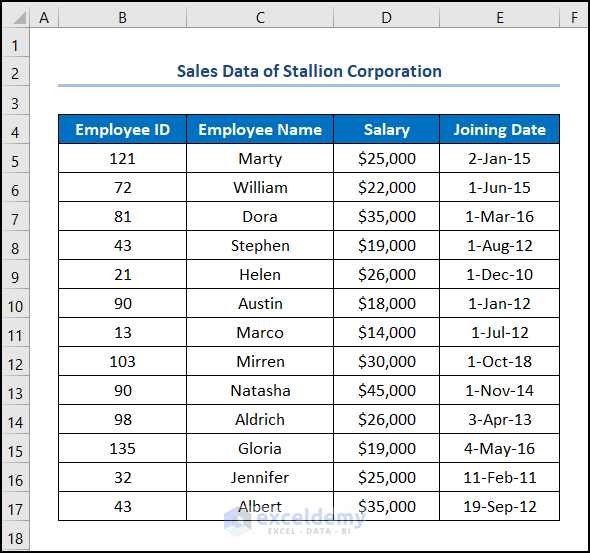
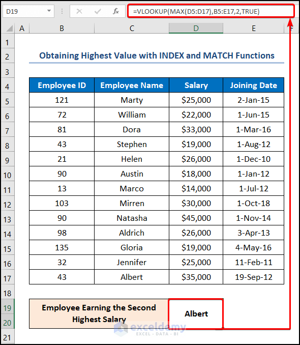
Suppose we have the Sales Data of Stallion Corporation dataset shown in the B4:E17 cells, which depicts the “Employee ID”, “Employee Name”, “Salary”, and “Joining Date” and want to get an employee with the highest ID and a salary above a $10k threshold.
Steps:
- Go to the D19 cell and enter the formula given below:
=VLOOKUP(MAXIFS(B5:B17,D5:D17,">10000"),B5:E17,2,FALSE)
Formula Breakdown:
- MAXIFS(B5:B17,D5:D17,”>10000″) → returns the maximum value among cells specific by a given set of criteria. Here, B5:B17 (max_range argument) is where the value is returned from. Next, the cells in D5:D17 (criteria_range argument) are being matched with “>10000” (criteria1 argument).
- Output → 135
- VLOOKUP(MAXIFS(B5:B17,D5:D17,”>10000″),B5:E17,2,FALSE) → becomes
- VLOOKUP(135,B5:E17,2,FALSE) → Here, 135 (lookup_value argument) is mapped from the B5:E17 (table_array argument) array. Next, 2 (col_index_num argument) represents the column number of the lookup value. Lastly, FALSE (range_lookup argument) refers to the Exact match of the lookup value.
- Output → Gloria
Read More: 10 Best Practices with VLOOKUP in Excel
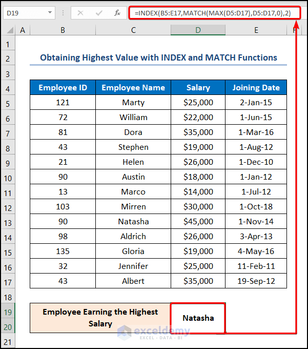
Alternative of VLOOKUP Function: Using INDEX-MATCH Formula to Get Highest Value
Steps:
- Go to D19 and apply the following formula:
=INDEX(B5:E17,MATCH(MAX(D5:D17),D5:D17,0),2)
Formula Breakdown:
- MAX(D5:D17) → for instance, the $B$5:$B$14 cells is the number1 argument which represents the “Total Point” column.
- Output → $45,000
- MATCH(MAX(D5:D17),D5:D17,0)→ In this formula, the MAX(D5:D17) cell points to the “Salary” of “$45,000”. Next, D5:D17 represents the array from which the “Salary” column where value is matched. Finally, 0 indicates the Exact match criteria.
- Output → 9
- INDEX(B5:E17,MATCH(MAX(D5:D17),D5:D17,0),2) → becomes
- INDEX(B5:E17,9,2) → returns a value at the intersection of a row and column in a given range. In this expression, the B5:E17 is the array argument which is the marks scored by the students. Next, 9 is the row_num argument that indicates the row location. Lastly, 2 is the optional column_num argument that points to the column location.
- Output → Natasha
How to Obtain the Next Highest Value with VLOOKUP
Steps:
- Jump to the D19 cell and type in the formula below:
=VLOOKUP(MAX(D5:D17),B5:E17,2,TRUE)
For example, the D5:D17 cells point to the “Salary” column.
Things to Remember
- The VLOOKUP function always looks for values from the leftmost top column to the right which means this function never fetches the data to the left.
- If you enter a value less than 1 as the column index number, the function will return an error.
- If there are multiple highest values in a worksheet, then the VLOOKUP function returns the first highest value in the list.
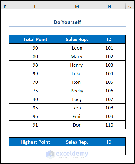
Practice Section
We have provided a Practice section on the right side of each sheet so you can practice yourself.
Download Practice Workbook
Further Readings
- How to Use VLOOKUP with Two Lookup Values in Excel
- How to Apply Double VLOOKUP in Excel?
- How to Use VLOOKUP Function with Exact Match in Excel
- How to Find Second Match with VLOOKUP in Excel
- VLOOKUP and Return All Matches in Excel
- VLOOKUP Fuzzy Match in Excel
- Excel VLOOKUP to Find Last Value in Column
- How to Use VLOOKUP to Search Text in Excel
- How to Apply VLOOKUP by Date in Excel
<< Go Back to VLOOKUP a Range | Excel VLOOKUP Function | Excel Functions | Learn Excel
Get FREE Advanced Excel Exercises with Solutions!

How do you use Vlookup and Max when the Matching value is in rows in the left column, but the data you want to analyze for the Max value is in columns D through O? Example, On Sheet 1 you have 10 Product names in Cells A2:A12. On Sheet 2, these same Product Names are listed in a table with Prices for each month of the year in columns D through O (columns B and C have other fixed data). The formula in Sheet 1 is to look for the product and then return the max price for the year by evaluating columns D through O in Sheet 2. I would like just one formula so that no matter what product is listed in Sheet 1, it will look at the correct row of data in sheet 2 and return the highest price listed for January through December (columns D through O).
Maybe it is not using VLookup and Max, but I’m not sure what functions to use.
Thank you
Hello ANDREW,
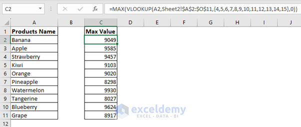
Hope you are doing well and thank you for your query. You can use VLOOKUP and MAX functions among other methods to look for a value when the value you want to analyze for is in columns D through O.
You can use the following formula.
=MAX(VLOOKUP(A2,Sheet2!$A$2:$O$11,{4,5,6,7,8,9,10,11,12,13,14,15},0))You can find the solution to your problem in the Excel file linked to this reply.
VLOOKUP and MAX to Look for Max Value
Regarding your query of product names changing in accordance with your changing the names in Sheet 1, you can use cell reference to copy the product names in Sheet 2. This will look for the correct row of data in Sheet 2.
Here is a screenshot of the results in the Excel file.
Hope you find this useful. Have a good day. Please let us know if you have any further queries. Also, you can post your Excel-related problems in the ExcelDemy Forum with images or Excel workbooks.
Regards,
ExcelDemy Team