The value of money is time-dependent. It changes with time. We often need to estimate the present value or future value of a certain amount of money. This can be easily done in Excel. Here, we will discuss the time value of money calculator in Excel in detail.
How to Make a Time Value of Money Calculator in Excel: 5 Handy Approaches
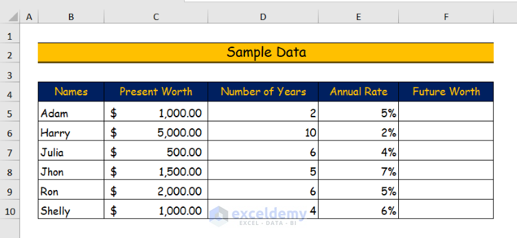
In this article, we will learn about five handy functions of Excel that are essential to calculating the time value of money. They are the PV function, the FV function, the RATE function, the NPER function, and finally the PMT function. We will use the dataset below to illustrate the methods.
1. Applying FV Function to Make a Time Value of Money Calculator in Excel
1.1 Estimating Future Values of Lump Sum
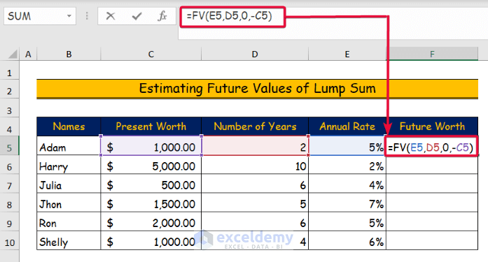
In this method illustration, we’ll use the FV function to estimate what a given sum of money will be worth in the future. Follow the outlined steps below to do the task.
Step 1:
- Firstly, select the cell where you want to calculate the future worth.
- In our case, we will select the F5 cell.
- Then, write down the following formula.
=FV(E5,D5,0,-C5)- Here, the first argument of the FV function is rate.
- So, we will select the E5 cell, which indicates rate.
- The next argument is nper, which indicates the number of periods.
- In our case, it is in cell D5.
- The third argument is pmt which means annual payment.
- In this instance, the annual payment is zero.
- The final argument is pv or present value.
- We will select the C5 cell.
- Finally, hit Enter.
Step 2:
- Consequently, we will see that the future value of the money will be in the cell.
- Then, move the cursor down to the last data cell.
- Excel will automatically fill the rest of the cells.
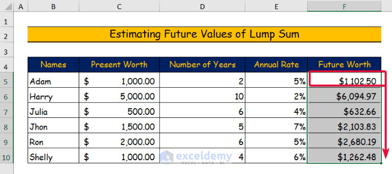
- We have added a minus sign before the value of the C5 cell or the present value.
- Since, we assumed that the present value is the amount deposited or paid into account. In other words cash outflow.
- As a result, we got the future value in plus sign according to convention. This indicates an increase in asset.
- We will continue this assumption throughout this article.
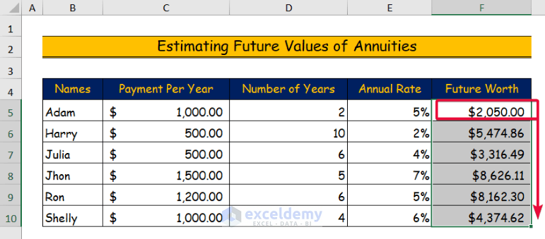
1.2 Estimating Future Values of Annuities
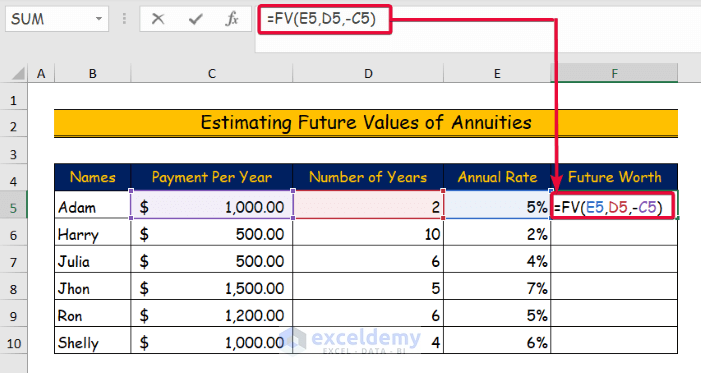
In this discussion, we will illustrate the use of the FV function to calculate the future value of a certain amount of money with a yearly payment. Follow the ensuing steps to complete the task.
Step 1:
- Firstly, choose the cell in which you want to determine the future value.
- In this case, we will select the F5 cell.
- Then, write down the following formula.
=FV(E5,D5,-C5)- The FV function’s first argument, in this case, is rate.
- Therefore, we will choose the rate-indicating E5 cell.
- The following argument is nper, which stands for “number of periods.”
- In this case, it is in cell D5.
- The third argument is pmt which means annual payment.
- In this instance, the annual payment is in cell C5.
- Finally, hit Enter.
Step 2:
- As a result, we will observe that the money’s future value is in the cell.
- After that, lower the cursor to the final data cell.
- The remaining cells will be automatically filled by Excel.
Read More: How to Calculate Future Value of Growing Annuity in Excel
2. Using PV Function to Make a Time Value of Money Calculator
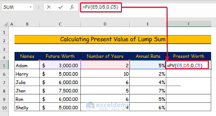
2.1 Calculating Present Value of Lump Sum
In this example, we’ll use the PV function to estimate the present value of a lump sum. Follow the sequential steps below to do that.
Step 1:
- Firstly, select the cell where you want to calculate the present value.
- In our case, we will go for the F5 cell.
- Then, write down the following formula.
=PV(E5,D5,0,C5)- rate serves as the PV function’s first argument in this instance.
- So, we’ll choose the rate-indicating E5 cell.
- The following argument, nper, specifies the number of periods.
- In this instance, it is in cell D5.
- .The third argument is pmt or annual payment.
- In this case, there is no yearly payment.
- The final argument is fv or future value.
- We will choose the C5 cell.
- Lastly, press Enter.
Step 2:
- As a result , we will see that the present worth of the money will be in the cell.
- Then, slide the cursor down to the last data cell.
- Excel will automatically complete the rest of the cells.
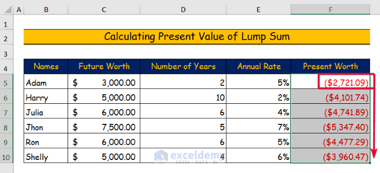
- We got the present value in red color which means cash outflow.
- Since we assumed the future value as cash inflow, we got the present value as cash outflow according to convention.
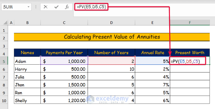
2.2 Calculating Present Value of Annuities
In this discussion, we will illustrate the use of the PV function to calculate the present value of a certain amount of money with a yearly payment. Follow the upcoming steps to complete the task.
Step 1:
- Firstly, decide which cell you want to use to calculate the present value.
- In this case, we will opt for the F5 cell.
- Then, write down the following formula.
=PV(E5,D5,C5)- In this case, rate is the first argument to the PV function.
- So, we’ll pick the E5 cell that indicates rate.
- nper, which stands for “number of periods”, is the next argument.
- In this instance, cell D5 contains it.
- The third argument is pmt which is nothing but an annual payment.
- In this instance, the annual payment is in cell C5.
- Finally, hit Enter.
Step 2:
- As a result, we will observe that the money’s present value is in the cell.
- After that, move the cursor down to the last data cell.
- Excel will subsequently fill in the remaining cells on its own.

Read More: How to Apply Present Value of Annuity Formula in Excel
3. Utilizing NPER Function to Make a Time Value of Money Calculator in Excel
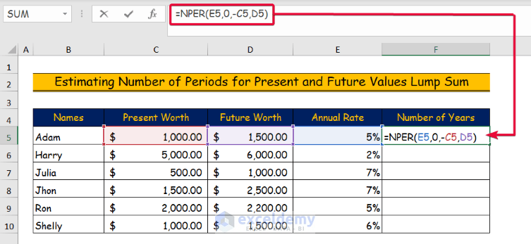
3.1 Estimating Number of Periods for Present and Future Values Lump Sum
In this method, we will calculate the number of periods needed to change the present value of a lump sum into a particular future value at a constant annual rate of return with the NPER function. Follow the steps that are coming up to do it.
Step 1:
- Firstly, decide which cell you want to use to calculate the number of periods.
- In this case, we will choose the F5 cell.
- Then, write down the following formula.
=NPER(E5,0,-C5,D5)- In this case, rate is the first argument to the NPER function.
- So, we’ll pick the E5 cell that contains the value of rate.
- pmt, which stands for “Annual Payment” is the next argument.
- In this case, it is zero.
- The third argument is pv or present value.
- In this instance, the present value is in cell C5.
- The final value is fv which is nothing but future value.
- Here, the D5 cell contains it.
- Finally, hit Enter.
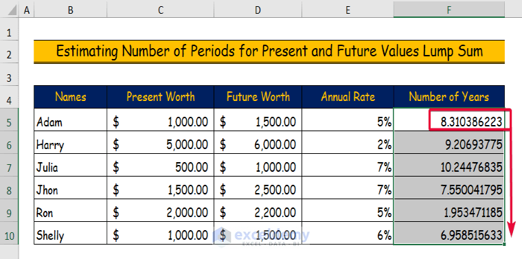
Step 2:
- As a result, we will observe the number of periods that appear in the cell.
- After that, slide the cursor down to the last data cell.
- Excel will subsequently complete the remaining cells on its own.
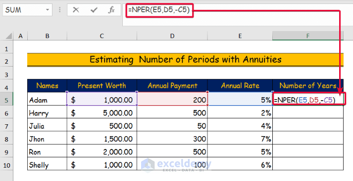
3.2 Estimating Number of Periods with Annuities
In this illustration of the method, we will calculate the number of periods needed to compensate a certain amount of money with a certain present value and a constant annual rate of return and annual payment. To complete the task, adhere to the given instructions.
Step 1:
- Firstly, decide which cell you want to use to calculate the number of periods.
- In this case, we will choose the F5 cell.
- Then, write down the following formula.
=NPER(E5,D5,-C5)- The NPER function’s first argument in this situation is rate.
- So, we’ll go for the E5 cell that contains values of rates.
- pmt, which is nothing but the annual payment is the next argument.
- In this case, it is in cell D5.
- The third argument is pv or present value.
- In this instance, the present value is in cell C5.
- Finally, hit Enter.
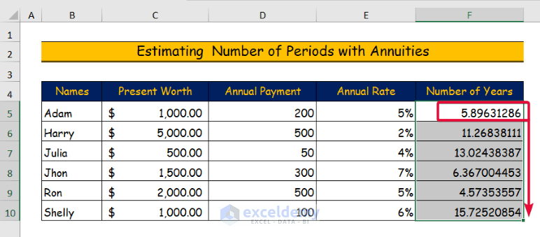
Step 2:
- Consequently, we will count the number of periods that appear in the cell.
- After that, move the cursor down to the final data cell.
- Excel will complete the remaining cells on its own.
Read More: How to Apply Future Value of an Annuity Formula in Excel
4. Using RATE Function to Make a Time Value of Money Calculator
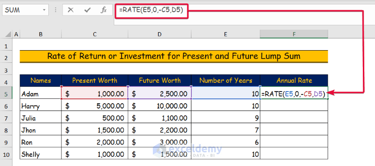
4.1 Rate of Return or Investment for Present and Future Lump Sum
In this instance, we will calculate the annual rate of return needed to change the present value of a certain amount of money to a particular future value for a certain number of periods. Follow the steps below to accomplish the deed.
Step 1:
- Firstly, select the cell that you want to use to calculate the annual rate.
- In this case, we will prefer the F5 cell.
- Then, write down the following formula.
=RATE(E5,0,-C5,D5)- In this case, nper is the first argument to the RATE function.
- So, we’ll opt for the E5 cell that contains values of number of periods.
- pmt, which indicates the annual payment is the next argument.
- In this case, the number of periods is zero.
- The third argument is pv or in other words present value.
- In this instance, the C5 cell holds the present value.
- The final argument is fv which is nothing but future value.
- Here, the D5 holds it.
- Finally, hit Enter.
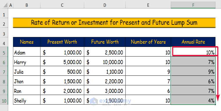
Step 2:
- As a result, we will observe that the annual rates will appear in the cell.
- After that, slide the cursor down.
- Excel will subsequently complete the remaining cells of the dataset.
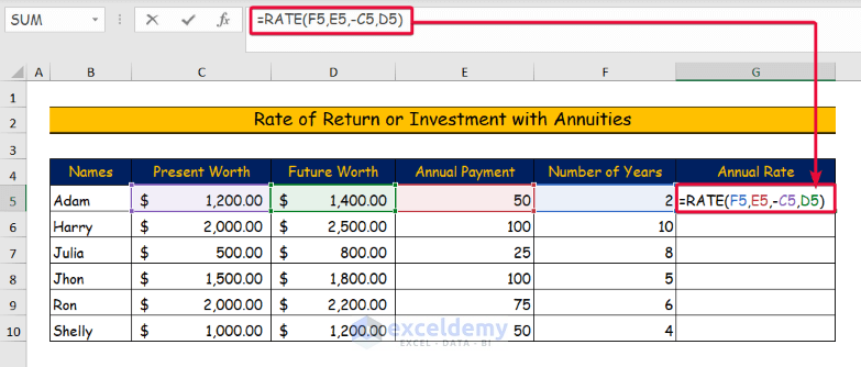
4.2 Rate of Return or Investment with Annuities
In this example, we will estimate the annual rate of return or investment. Follow the sequentially outlined steps below.
Step 1:
- Firstly, decide which cell you want to use to calculate annual rates.
- In this case, we will pick the F5 cell.
- Then, write down the following formula.
=RATE(F5,E5,-C5,D5)- In this case, the first argument to the RATE function is nper or the number of periods.
- So, we’ll go for the E5 cell that contains the value for the number of periods.
- pmt or the annual payment is the next argument.
- In this case, it is in cell E5.
- pv, or present value, is the third argument.
- In this instance, the present value is contained in cell C5.
- The final value is fv which means the future value.
- Here, the D5 cell holds it.
- Finally, press Enter.
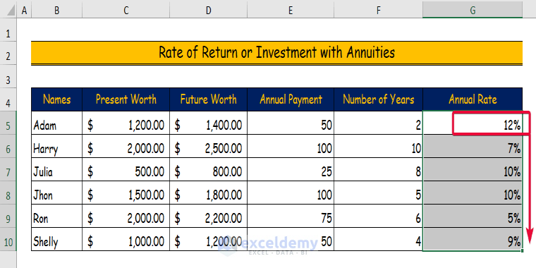
Step 2:
- Consequently, we will observe the rate that appear in the cell.
- After that, the cursor goes down to the final data cell.
- The remaining cells will be filled out by Excel on its own.
Read More: How to Calculate Present Value of Lump Sum in Excel
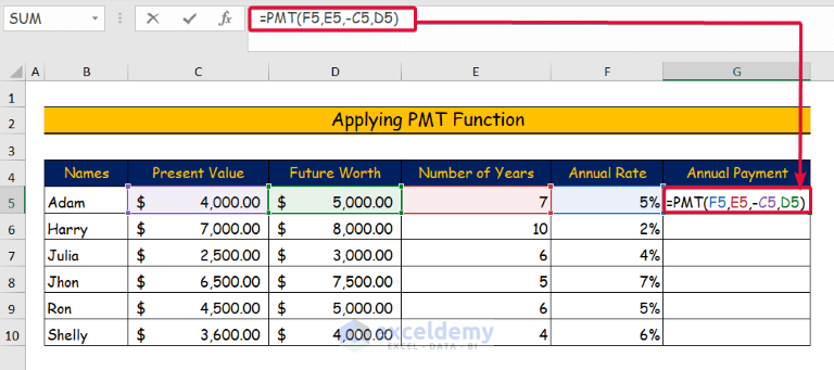
5. Applying PMT Function to Make a Time Value of Money Calculator in Excel
In this method, we will estimate the annual payment for a certain investment. Adhere to the following steps to do it.
Step 1:
- Firstly, select the cell that you want to use to calculate the annual payment.
- In this case, we will prefer the G5 cell.
- Then, write down the following formula.
=PMT(F5,E5,-C5,D5)- In this case, rate is the first argument to the PMT function.
- So, we’ll opt for the F5 cell that contains values of number of periods.
- pmt, which indicates the nper or the number of periods is the next argument.
- In this case, the value of the number of periods is in cell E5.
- pv or present value is the third argument.
- In this instance, the C5 cell holds the present value.
- The last argument is fv which is nothing but future value.
- Here, the value is in the D5 cell.
- Finally, hit Enter.
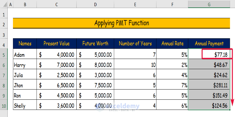
Step 2:
- As a result, we will observe that the annual payment will appear in the cell.
- After that, slide the cursor down to the final data cell.
- Excel will subsequently enter the values of the remaining cells of the dataset.
Read More: How to Calculate Present Value in Excel with Different Payments
Download the Practice Workbook
Conclusion
The time value of money calculator is an important tool in the financial sector as well as in our daily life. This allows us to predict the future value of a present sum of money and vice versa. In this article, we have discussed how such a calculator can be easily made in Excel. This will allow Excel users to evaluate the time value of money properly. If you find it useful, please let us know in the comment section below and share any recommendations and thoughts regarding this or any other content of ours. T
Related Articles
- How to Calculate Future Value in Excel with Different Payments
- How to Calculate Present Value of Future Cash Flows in Excel
- How to Calculate Future Value of Uneven Cash Flows in Excel
- How to Calculate Present Value of Uneven Cash Flows in Excel
- How to Calculate Future Value with Inflation in Excel
- Calculate NPV for Monthly Cash Flows with Formula in Excel
<< Go Back to Time Value Of Money In Excel | Excel for Finance | Learn Excel
Get FREE Advanced Excel Exercises with Solutions!
