Sometimes, when filling out a form in Excel, the data entry cells may be scattered across the worksheet. Therefore, we want an easy way to go through the cells in the correct order. Moreover, we often need to create worksheets for other users in Excel. It would be great if we could make the worksheet in such a way that when they enter data in one cell, they can quickly move on to the next. In this article, we are going to learn how to tab to certain cells in Excel.
How to Tab to Certain Cells in Excel: 2 Easy Ways
Here, we are going to discuss two easy ways to tab to certain cells in Excel with some beautiful examples and explanations. These techniques will guide us to jump to the next data entry cell. Most importantly, we can tab certain cells only when the worksheet is normal. If the worksheet is protected, then we need to unlock the cells first. So without further delay, let’s get started.
1. Tab to Certain Cells Using Keyboard Shortcut in Excel
In this method, we will learn to tab to certain cells by using keyboard shortcuts in Excel. Hence, this is a very quick method to jump to the next data entry cell. Here, we will discuss two ways of using the keyboard shortcut for the task. The steps for these two ways are below.
1.1 Tab to Next Entry Cell
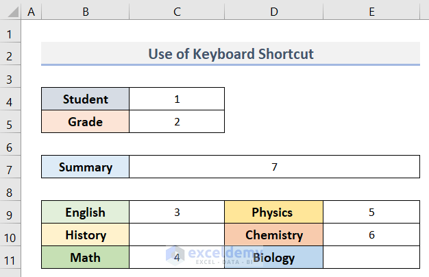
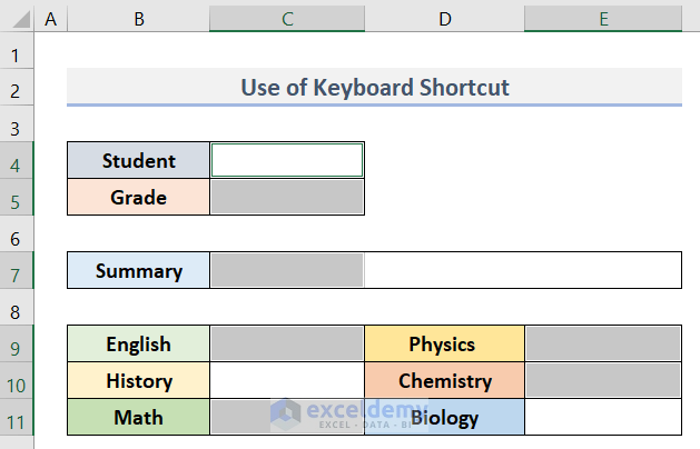
Suppose, we have a dataset (B4:E11) in Excel that contains the Name and Grades of some subjects of a student. In the screenshot below, we can see the report card with some cells with numbers (1, 2, 3, 4, 5, 6, 7) which indicate the order of data entry. The steps to tab these cells in a specific order are below.
Steps:
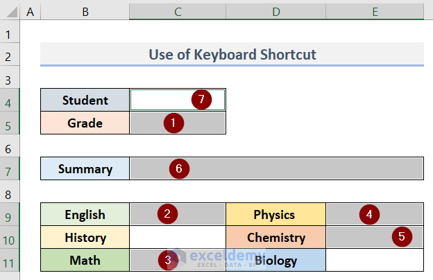
- Firstly, choose the second cell into which you want to enter information. In our case, we have selected cell C5 first where we will enter the Grade level of the student.
- Next, while holding down the Ctrl key, select the next cell, then the next, until all of the resting cells (3-7) are chosen.
- Eventually, choose the first cell of the order- in this case, cell C4.
- As cell C4 was chosen last, it is now the functioning cell of the range.
- When we use this range in the future, we’ll start from cell C4. For a better understanding of the order of selection of cells, see the screenshot below.
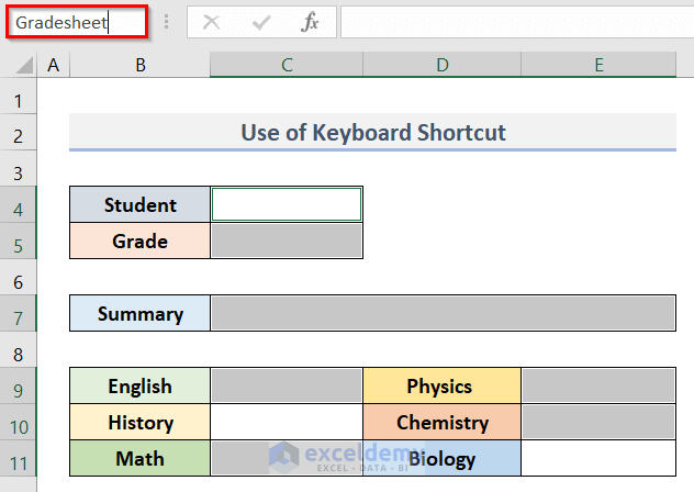
- Now, we need to give the chosen cells a name. To do so, while selecting the cells, click on the Name box. We can see the position of the box in the picture below.
- Subsequently, give this group of cells a one-word name. In our case, we have used ‘Gradesheet’ as the name of the cells.
- In the end, to save the name, press the Enter button.
Consequently, if we need to enter data into the cells, we can easily choose the named range and navigate through the cells. The steps of this task are below:
- In the first place, click the drop-down arrow to the right side of the Name box.
- Secondly, select the name you gave it. In our case, we have selected ‘Gradesheet’.
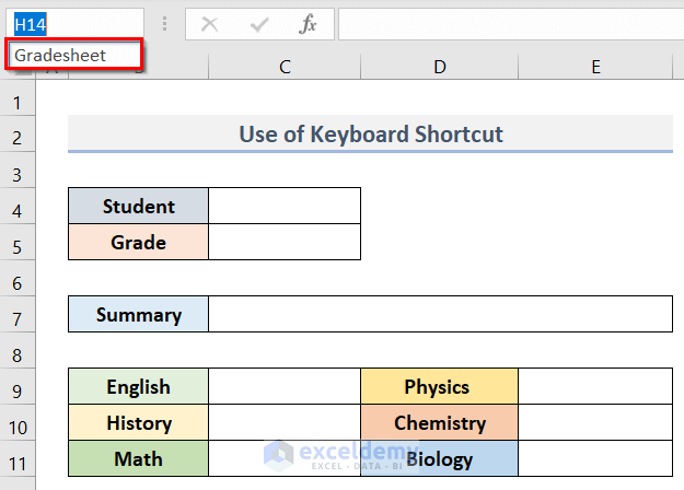
- As a result, the range of cells of the names is selected.
- After selecting the range, type in the cell that is functioning (cell C4 in our case).

- In turn, to move to the next cell, press the Tab or Enter key. We can see the result in the screenshot below.

- Similarly, after typing in the second cell we will move to the third cell (C9) of the range and it will continue in a loop.

- In this way, we can type according to our selection in the dataset. When all of the cells have been done, click a cell other than the named range to deselect it.

1.2 Jump to Next Blank Cell
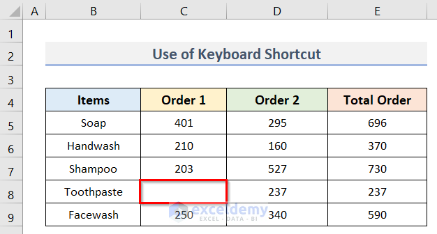
Assuming, we have a dataset (B4:E9) in Excel that contains the names and Orders and Total Order of some Items. We can see in the screenshot below that cell C8 is blank. Now, by following some easy steps, we can jump to the blank cell.
Steps:
- In the beginning, select the heading of the column (C4) where the blank cell is.
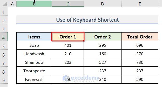
- Then, press the Alt + Down Arrow Key on the keyboard.
- Therefore, we will jump to the cell (C7) just upward to the blank cell (C8).
- Thus, we can move to the blank cell so easily.

Read More: How to Shift Cells Down in Excel
2. Apply Excel VBA to Tab Order of Certain Cells
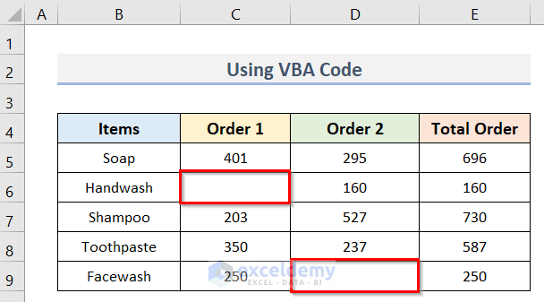
We can also use Excel VBA to tab the order of certain cells. Let’s say, we have a dataset (B4:E9) in Excel where we can see two blank cells which are: cells C6 and D9. Assuming we want to create a tab order from cell C6 to cell D9. Here, we will use Excel VBA to jump to the blank cells according to the tab order. The steps to do so are below.
Steps:
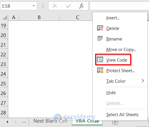
- Firstly, right-click on the sheet tab (VBA Code) below the worksheet and select View Code in the context menu.
- Then, a Microsoft Visual Basic for Applications window will pop up.
- Now, copy the VBA code below and paste it into the Code window.
Private Sub Worksheet_Change(ByVal Target As Range)
Dim tArray As Variant
Dim j As Long
tArray = Array("C6", "D9")
Application.ScreenUpdating = False
For j = LBound(tArray) To UBound(tArray)
If tArray(j) = Target.Address(0, 0) Then
If j = UBound(tArray) Then
Me.Range(tArray(LBound(tArray))).Select
Else
Me.Range(tArray(j + 1)).Select
End If
End If
Next j
Application.ScreenUpdating = True
End Sub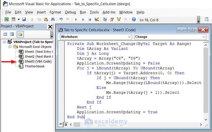
Notes:
- The order of the input cells in the code is C6, D9 and we have to use the uppercase letter for the cell address.
- Besides, we must unlock the input cells for the protected worksheet.
- Eventually, close the Microsoft Visual Basic for Applications window by pressing the Alt + Q keys.
- Therefore, select the first cell (C6) of order and input data.

- After entering data in C6, the cursor will now move to D9 when you press the Tab or Enter We can see that in the picture below.

- Finally, when we press Enter after entering data in cell D9, automatically cell C6 will be selected again.

Read More: How to Move Down One Cell Using Excel VBA
Download Practice Workbook
Download the practice workbook from here.
Conclusion
I hope the above methods will be helpful for you to tab to certain cells in Excel. Download the practice workbook and give it a try. Let us know your feedback in the comment section.
Related Articles
- How to Shift Cells Up in Excel
- How to Shift Cells Down in Excel without Changing Formula
- How to Shift Cells Right in Excel
- Fix: Excel Cannot Shift Nonblank Cells
- How to Perform Double Click Cell Jump in Excel
- Move One Cell to Right Using VBA in Excel
<< Go Back to Move Cells | Excel Cells | Learn Excel
Get FREE Advanced Excel Exercises with Solutions!
