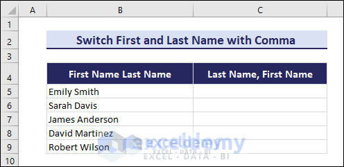
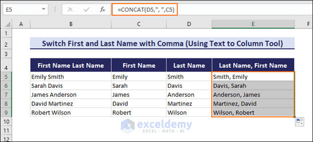
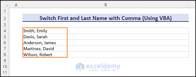
In this Excel tutorial, you will learn how to switch first and last name in Excel with comma. For example, you have a name like this: Emily Smith, and you want to convert this to: Smith, Emily. In the following image, you see, that we have switched the first and last name in Excel with comma.

Switching first name and last name in Excel using Flash Fill feature.
Switching First and Last name in Excel with comma can be done by several ways: using Excel Flash Fill feature (the easiest method); combining different Excel functions; using Convert Text to Columns Wizard; using Power Query; using Power Pivot; and applying Excel VBA code.
Generally, we need to switch first and last name with comma for documentation or official purposes. If you have to switch first and last name with comma for a large dataset, using Excel would be really handy.
We will use the following dataset to show how to switch first and last name in Excel with a comma. Here, column B contains the first and last names of 5 people. Our goal is to switch the first name and last name with a comma. For example, Emily Smith will be Smith, Emily.
1.Using Flash Fill feature to Switch First and Last Name in Excel with Comma
Excel’s Flash Fill feature is the easiest way to reverse the first name and last name in Excel with comma.
Flash Fill feature automatically fills in values according to a specific pattern you provide. You have to provide it with an example to recognize the pattern but sometimes you need to provide it with a couple of examples (when dataset is complex) to recognize the pattern that you want as output.
We shall use the Flash Fill feature in two ways to switch first and last name in Excel with comma. The first way is using Flash Fill from the Home tab, and another way is using it from the Fill Handle tool. Let’s start with using the Flash Fill option from the Home tab to switch first and last name with comma.
1.1 Using Flash Fill Option from the Home Tab
In this part, we shall use the Flash Fill option which is under the Editing group of commands of the Home tab. We will use the previously mentioned dataset. Follow the steps:
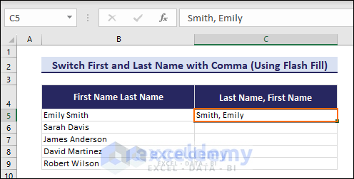
Step 1: Select cell C5 and input the name like this: Smith, Emily.

Note: Be careful about the consistency of the pattern in your data. For example, you must have only the First Name and Last Name in cells. If all the cells don’t have a similar pattern, then Flash Fill won’t identify the pattern correctly. That will result in giving wrong outputs. So, it’s a good practice to cross-check the data.
Step 2: Go to the Home tab => Editing group of commands => Click on the Fill dropdown =>You will get the Flash Fill command.
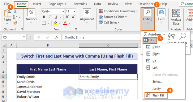
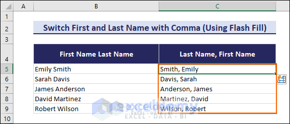
Step 3: Click on the Flash Fill option and you will get the First Name Last Name switched to format Last Name, First Name.
Note:
1. You can also choose the Flash Fill option from here:
Data tab => Data Tools group of commands => Flash Fill
2. Alternatively, you can use the keyboard shortcut Ctrl+E for Flash Fill.
=> Select cell C5 and input the name like this: Smith, Emily
=> Keeping cell C5 selected, press Ctrl+E on the keyboard. You will get the First Name and Last Name switched with a comma.
1.2 Using Flash Fill from the Fill Handle tool to Swich First Name and Last Name in Excel
In this step, we shall use Excel’s Flash Fill to switch names but we shall use Flash Fill with Excel’s other popular feature Fill Handle.
Follow these steps. We have the same dataset.
Step 1: Select cell C5 and input the name like this: Smith, Emily.
Step 2: Now I take my mouse over the bottom-right corner of the cell C5.
=> The cursor will be changed from the White Plus sign to Green Plus. This Green Plus is our Fill Handle feature.
=> Now click and drag the mouse until the mouse reaches the last row of the data
=> You will find the Auto Fill Options drop-down icon, click on the icon, you will get several options displayed. Choose the last one, Flash Fill. You will get the desired output. First Name Last Name to Last Name, First Name for the whole data.
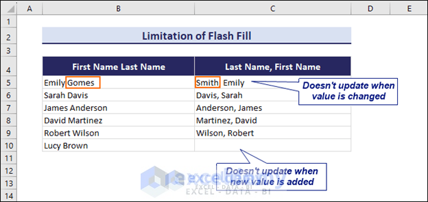
Note: The Flash Fill method is not dynamic. If you change the original data, then the cells where you used Flash Fill will not be changed automatically. You have to reuse Flash Fill after changing any data.
For example, we have changed the cell B5 from Emily Smith to Emily Gomes. However, the C5 cell of the column, where we applied Flash Fill is not updated according to the changed data. If you add a new value to the original dataset, Flash Fill won’t work for the newly added data. Follow the image below:
Because of the static nature of the Flash Fill feature, it is not feasible for changeable data. We will use combinations of Excel functions to switch first and last name in Excel with comma. If you apply the following formulas, your data will be updated automatically, whenever you make any changes to the original data.
2. Using Excel Formulas to Switch First and Last Name in Excel with Comma
Using Excel formulas is definitely a dynamic fix to switch first and last name with comma.
Excel doesn’t have any specific function that will switch the first and last names with a comma. So, we shall use combined functions. We shall use functions like RIGHT, LEFT, LEN, MID, SEARCH, FIND, SUBSTITUTE, CONCAT, REPLACE, etc. to do this.
Here, you will learn 9 formulas to switch first and last name in Excel with comma. Each formula will contain combined functions. Let’s start with using RIGHT, LEN, SEARCH, and LEFT functions to create a formula.
2.1 Combining RIGHT, LEN, SEARCH, and LEFT Functions
In this section, we shall combine the RIGHT, LEN, SEARCH, and LEFT text functions to switch first and last names with commas. These functions will work together to return the desired result.
Follow the steps:
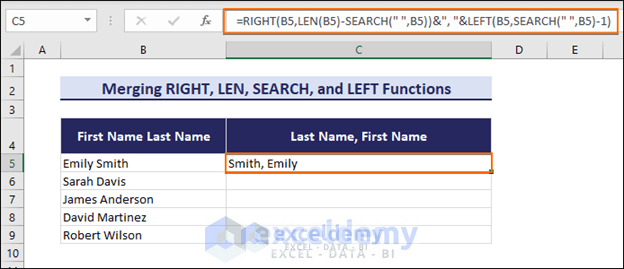
Step 1: Write this formula in cell C5 and press the Enter button.
=RIGHT(B5,LEN(B5)-SEARCH(" ",B5))&", "&LEFT(B5,SEARCH(" ",B5)-1)You will get the desired output: Smith, Emily in cell C5.
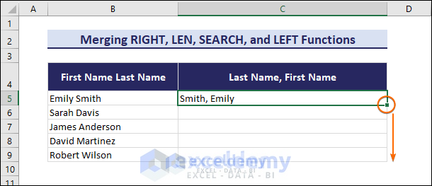
Step 2: Take the mouse over the bottom-right corner of the cell C5.
=> The cursor will be changed from the White Plus sign to Green Plus. This Green Plus is our Fill Handle feature.
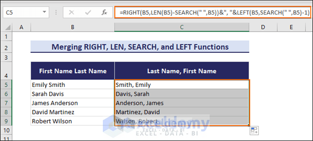
Drag the Fill Handle and AutoFill the formulas up to the last row of data.
We have switched the first and last names with commas for the rest of the cells.
Let’s explain how this formula works:
=RIGHT(B5,LEN(B5)-SEARCH(” “,B5))&”, “&LEFT(B5,SEARCH(” “,B5)-1)
=RIGHT(B5,LEN(B5)-SEARCH(” “,B5))&”, “&LEFT(B5,6-1)// SEARCH(” “,B5) returns 6 because it searched for a space in cell B5 and the space is found at the 6th position.
=RIGHT(B5,LEN(B5)-SEARCH(” “,B5))&”, “&“Emily”//LEFT(B5,6-1) returns “Emily” because in cell B5, the first 5 (6-1=5) characters from left is “Emily”
=RIGHT(B5,LEN(B5)–6)&”, “&”Emily”// SEARCH(” “,B5) returns 6 because it searched for a space in cell B5 and it is found at the 6th position.
=RIGHT(B5,11-6)&”, “&”Emily”// LEN(B5) returns 11 because the length of the cell B5 is 11 including the space.
=“Smith”&”, “&”Emily”// RIGHT(B5,11-6) returns “Smith” because in cell B5, the first 5 (11-6=5) characters from right is “Smith”
=Smith, Emily // the ampersand signs join the results with a comma between them.
Note: Be aware of the extra spaces in the original dataset. This formula works by searching a single space between the first and last name. So, if your data contains more than one space between the first and last names, it will give an incorrect result. You can use the TRIM function to eliminate the extra spaces. Just use TRIM(B5) instead of B5 in the above formula.
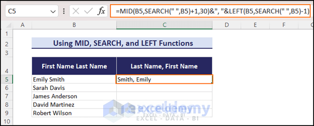
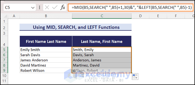
2.2 Using MID, SEARCH, and LEFT Functions
In this section, we shall combine the MID, SEARCH, and LEFT text functions to switch first and last names with commas. These functions will work together to return the correct result.
Follow the steps:
Step 1: Copy this formula in cell C5 and hit the Enter key.
=MID(B5,SEARCH(" ",B5)+1,30)&", "&LEFT(B5,SEARCH(" ",B5)-1)Right after pressing Enter, you will get the output: Smith, Emily in cell C5. Here, the first and last name will switch with a comma between them.
Step 2: To get the results for the other cells, drag the Fill Handle and AutoFill the formulas up to the last row of data.
Therefore, you will get the results for rest of the cells.
=MID(B5,SEARCH(” “,B5)+1,30)&”, “&LEFT(B5,SEARCH(” “,B5)-1)
=MID(B5,SEARCH(” “,B5)+1,30)&”, “&LEFT(B5,6-1) // SEARCH(” “,B5) returns 6 because it searched for a single space in cell B5 and it found the space at the 6th position.
=MID(B5,SEARCH(” “,B5)+1,30)&”, “&“Emily”// LEFT(B5,6-1) returns “Emily” because in cell B5, the first 5 (6-1=5) characters from left is “Emily”
=MID(B5,6+1,30)&”, “&”Emily”// SEARCH(” “,B5) returns 6 because it searched for a space in cell B5 and it is found at the 6th position.
=“Smith”&”, “&”Emily”// MID(B5,6+1,30) returns “Smith” because it returns the strings of cell B5 starting from the 7th (6+1=7) position up to 30th position. As we want the strings up to the last character of cell B5, we provided an assumed number 30 here.
=Smith, Emily // the ampersand signs join the results with a comma between them.
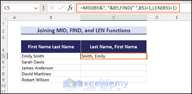
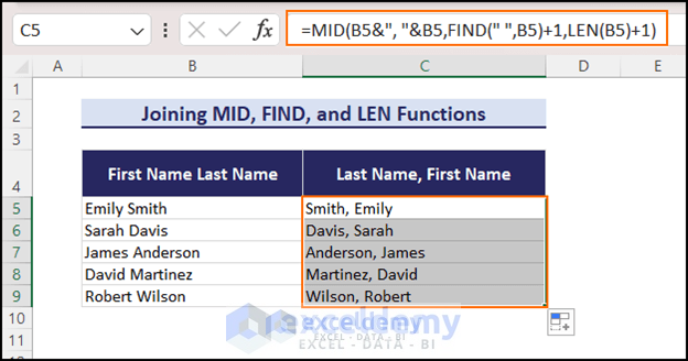
2.3 Joining MID, FIND, and LEN Functions
Joining MID, FIND, and LEN text functions is an easy yet dynamic fix to switch the first and last names with commas.
Follow the steps:
Step 1: Write this formula in cell C5 and click on the Enter key.
=MID(B5&", "&B5,FIND(" ",B5)+1,LEN(B5)+1)The result will be: Smith, Emily in cell C5. You will get the first and last name switched with a comma.
Step 2: Now, to get the outputs for the other cells, drag the Fill Handle and AutoFill the formulas up to the last row of data.
You will get the first and last names switched with a comma for the entire dataset.
=MID(B5&”, “&B5,FIND(” “,B5)+1,LEN(B5)+1)
=MID(B5&”, “&B5,FIND(” “,B5)+1,11+1)// LEN(B5) returns 11 because the length of the cell B5 is 11 including the space.
=MID(B5&”, “&B5,6+1,11+1)// FIND(” “,B5) returns 6 because the FIND functions found a single space in cell B5 at the 6th position.
=“Smith, Emily“// MID(B5&”, “&B5,6+1,11+1) returns “Smith, Emily” because the MID function concatenated the value of B5 cell with a comma and a space with the same value of cell B5 from 7th (6+1=7) to 12th (11+1=12) position.
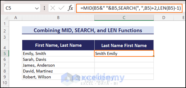
2.4 Combining MID, SEARCH, and LEN Functions
In this portion, we shall combine the MID, SEARCH and LEN functions to switch the first and last name in Excel without a comma.
For example, Smith, Emily will be Emily Smith.
Follow the steps:
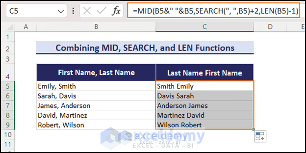
Step 1: Copy this formula in cell C5 and hit the Enter button.
=MID(B5&" "&B5,SEARCH(", ",B5)+2,LEN(B5)-1)Therefore, you will get the desired output in cell C5: Smith Emily
Step 2: To switch the first and last names without commas for the rest of the cells, drag the Fill Handle and AutoFill the formulas up to the last row of data.
So, you will get the results for the entire dataset.
=MID(B5&” “&B5,SEARCH(“, “,B5)+2,LEN(B5)-1)
=MID(B5&” “&B5,SEARCH(“, “,B5)+2,12-1)// LEN(B5) returns 12 because the length of the cell B5 is 12 including the comma and the space.
=MID(B5&” “&B5,6+2,12-1)// SEARCH(“, “,B5) returns 6 because it searched for a comma followed by a space in cell B5 and found it at 6th position.
=Smith Emily// MID(B5&” “&B5,6+2,12-1) returns Smith Emily because the MID function concatenated the value of B5 with a space and with the value of cell B5 from 8th (6+2=8) to 11th (12-1=11) position.
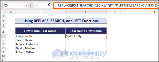
2.5 Using REPLACE, SEARCH, and LEFT Functions
In this section, we shall use the REPLACE, SEARCH, and LEFT text functions to switch first and last name in Excel without comma.
Let’s follow the steps:
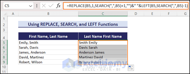
Step 1: Write this formula in cell C5 and press Enter.
=REPLACE(B5,1,SEARCH(",",B5)+1,"")&" "&LEFT(B5,SEARCH(",",B5)-1)Therefore, you will get the first and last names switched without comma. In other words, you will get: Smith Emily in cell C5.
Step 2: Drag the Fill Handle and AutoFill the formulas up to the last row of data. You will get the desired outputs for the rest of the cells.
=REPLACE(B5,1,SEARCH(“,”,B5)+1,””)&” “&LEFT(B5,SEARCH(“,”,B5)-1)
=REPLACE(B5,1,SEARCH(“,”,B5)+1,””)&” “&LEFT(B5,6-1)// SEARCH(“, “,B5) returns 6 because it searched for a comma in cell B5 and found it at 6th position.
=REPLACE(B5,1,SEARCH(“,”,B5)+1,””)&” “&“Emily”// LEFT(B5,6-1) returns “Emily” because in cell B5, the first 5 (6-1=5) characters from left is “Emily”.
=REPLACE(B5,1,6+1,””)&” “&”Emily” // SEARCH(“,”,B5)+1 returns 6 because the position of the space in cell B5 is found at 6th position.
=“Smith“&” “&”Emily”// REPLACE(B5,1,6+1,””) returns “Smith” because it replaces 1st to 7th (6+1=7) character of cell B5 with no space (“”). If “Emily, ” is replaced with no space, “Smith” will remain.
=Smith Emily// the ampersand signs join the results with a comma between them.
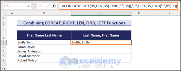
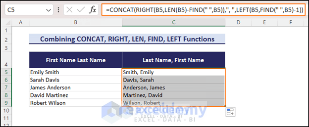
2.6 Combining CONCAT, RIGHT, LEN, FIND, and LEFT Functions
We shall combine the CONCAT, RIGHT, LEN, FIND, and LEFT functions to reverse the first and last name in Excel with comma.
Follow the steps:
Step 1: Write this formula in cell C5.
=CONCAT(RIGHT(B5,LEN(B5)-FIND(" ",B5)),", ",LEFT(B5,FIND(" ",B5)-1))Press the Enter button and you will get the output: Smith, Emily in cell C5.
Step 2: Now, drag the Fill Handle and AutoFill the formulas up to the last row of data. Thus you will switch the first and last names with comma for all cells.
=CONCAT(RIGHT(B5,LEN(B5)-FIND(” “,B5)),”, “,LEFT(B5,FIND(” “,B5)-1))
=CONCAT(RIGHT(B5,LEN(B5)-FIND(” “,B5)),”, “,LEFT(B5,6-1))// FIND(” “,B5) returns 6 because the FIND functions found a single space in cell B5 at the 6th position.
=CONCAT(RIGHT(B5,LEN(B5)-FIND(” “,B5)),”, “,”Emily“)// LEFT(B5,6-1) returns “Emily” because in cell B5, the first 5 (6-1=5) characters from left is “Emily”.
=CONCAT(RIGHT(B5,LEN(B5)–6),”, “,”Emily”)// FIND(” “,B5) returns 6 because the FIND functions found a single space in cell B5 at the 6th position.
=CONCAT(RIGHT(B5,11-6),”, “,”Emily”)// LEN(B5) returns 11 because the length of the cell B5 is 11 including the space.
=CONCAT(“Smith“,”, “,”Emily”)// RIGHT(B5,11-6) returns “Smith” because in cell B5, the first 5 (11-6=5) characters from right is “Smith”
=Smith, Emily// CONCAT(“Smith”,”, “,”Emily”) returns Smith, Emily because it concatenated the values “Smith”, “, ”, and “Emily”.
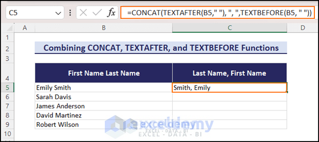
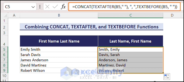
2.7 Joining CONCAT, TEXTAFTER, and TEXTBEFORE Functions
In this section, we shall join the CONCAT, TEXTAFTER, and TEXTBEFORE functions to switch the first and last names with comma.
Note: The TEXTAFTER and TEXTBEFORE functions are only available in the Microsoft 365 version.
Let’s follow the steps:
Step 1: Copy this formula in cell C5 and hit the Enter button.
=CONCAT(TEXTAFTER(B5," "), ", ",TEXTBEFORE(B5, " "))Thus you will get the first and last names switched with a comma: Smith, Emily in cell C5.
Step 2: To get the values for the rest of the cells, drag the Fill Handle and AutoFill the formulas up to the last row of data.
You will get the outputs for the rest of the cells.
=CONCAT(TEXTAFTER(B5,” “), “, “,TEXTBEFORE(B5, ” “))
=CONCAT(TEXTAFTER(B5,” “), “, “,”Emily“)// TEXTBEFORE(B5, ” “) returns “Emily” because the text before a space in cell B5 is “Emily”.
=CONCAT(“Smith“, “, “,”Emily”)// TEXTAFTER(B5,” “) returns “Smith” because the text after a comma followed by a space in cell B5 is “Smith”.
=Smith, Emily// CONCAT(“Smith”, “, “,”Emily”) returns “Smith, Emily” because it concatenated the values “Smith”, “, ” and “Emily”.
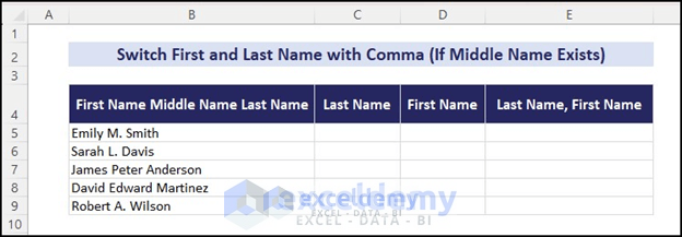
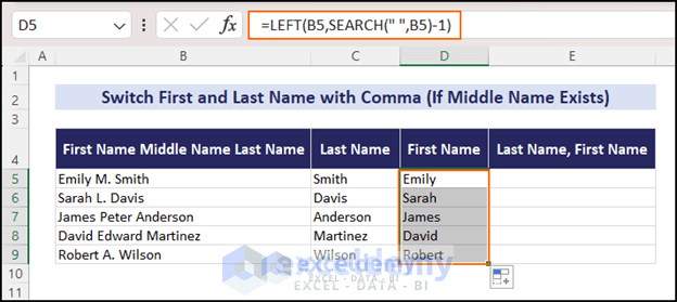
2.8 Using RIGHT, LEFT, LEN, SEARCH, SUBSTITUTE, and CONCAT Function (If Middle Name is Present)
In this section, we shall learn how to switch first and last name with comma if the names contain middle names also. We shall combine the RIGHT, LEFT, LEN, SEARCH, SUBSTITUTE, and CONCAT functions to do this task.
First, we shall extract the last name and first name in C and D columns by using combined functions. Then, by using the CONCAT function, we shall join the last name and first name with a comma.
We shall use the following dataset.
Follow the steps:
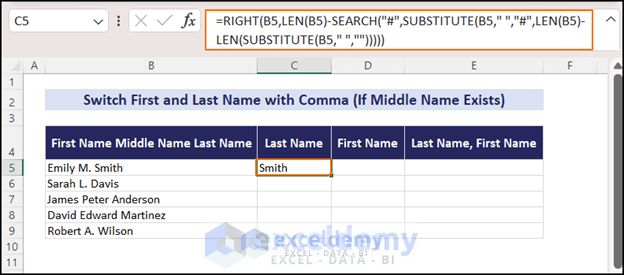
Step 1: To get the last names, write this formula in cell C5 and press Enter.
=RIGHT(B5,LEN(B5)-SEARCH("#",SUBSTITUTE(B5," ","#",LEN(B5)-LEN(SUBSTITUTE(B5," ","")))))You will get the last name: Smith in cell C5.
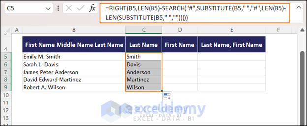
Step 2: Drag the Fill Handle and AutoFill the formulas up to the last row of data.
Therefore, you will get the last names for the entire dataset.
=RIGHT(B5,LEN(B5)-SEARCH(“#”,SUBSTITUTE(B5,” “,”#”,LEN(B5)-LEN(SUBSTITUTE(B5,” “,””)))))
=RIGHT(B5,LEN(B5)-SEARCH(“#”,SUBSTITUTE(B5,” “,”#”,LEN(B5)-LEN(“EmilyM.Smith“))))// SUBSTITUTE(B5,” “,””) returns EmilyM.Smith because it substituted the spaces of cell B5 with no space.
=RIGHT(B5,LEN(B5)-SEARCH(“#”,SUBSTITUTE(B5,” “,”#”,LEN(B5)–12)))// LEN(“EmilyM.Smith”) returns 12 since the length of “EmilyM.Smith” is 12.
=RIGHT(B5,LEN(B5)-SEARCH(“#”,SUBSTITUTE(B5,” “,”#”,14-12)))// LEN(B5) returns 14 because the length of the characters of cell B5 is 14 including the spaces.
=RIGHT(B5,LEN(B5)-SEARCH(“#”,“Emily M.#Smith”))// SUBSTITUTE(B5,” “,”#”,14-12) returns “Emily M.#Smith” because it substituted the space with “#” at 2nd (14-12=2) instance.
=RIGHT(B5,LEN(B5)–9)// SEARCH(“#”,”Emily M.#Smith”) returns 9 because it searched the position of “#” and it is at 9th position.
=RIGHT(B5,14-9)// LEN(B5) returns 14 because it is the length of cell B5.
=Smith// RIGHT(B5,14-9) returns “Smith” because from right, “Smith” is the 5 (14-9=5) strings.
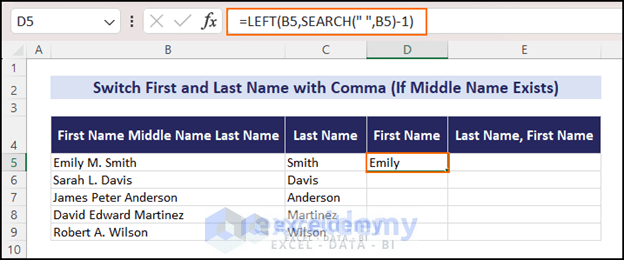
Step 3: To get the first names, write this formula in cell D5 and press Enter.
=LEFT(B5,SEARCH(" ",B5)-1)Thus you will get the first name: Emily in cell D5.
Step 4: Drag the Fill Handle and AutoFill the formulas up to last row of data.
You will get the first names for the rest of the cells.
=LEFT(B5,SEARCH(” “,B5)-1)
=LEFT(B5,6-1)// SEARCH(” “,B5) returns 6 because the first space is at 6th position in cell B5.
=Emily// LEFT(B5,6-1) returns “Emily” because it is the first 5 (6-1=5) characters from left in cell B5.
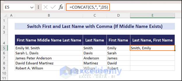
Step 5: Now, we shall join the last and first name with comma. Write this formula in cell E5 and press Enter.
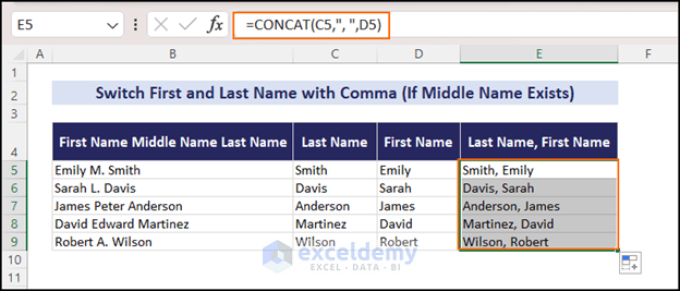
=CONCAT(C5,", ",D5)You will get the output: Smith, Emily in cell E5. So, the first and last name is switched with comma.
Step 6: Drag the Fill Handle and AutoFill the formulas up to last row of data.
Therefore, you will get the output for the rest of the cells.
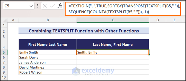
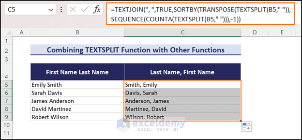
2.9 Using TEXTSPLIT Function with Other Functions
In this portion, we shall combine the TEXTSPLIT function with other functions TEXTJOIN, SORTBY, TRANSPOSE, SEQUENCE, and COUNTA to switch first and last name in Excel with comma.
We shall use the same dataset. Follow the steps:
Step 1: Write this formula in cell C5 and hit the Enter button.
=TEXTJOIN(", ",TRUE,SORTBY(TRANSPOSE(TEXTSPLIT(B5," ")),SEQUENCE(COUNTA(TEXTSPLIT(B5," "))),-1))Thus, you will get the output: Smith, Emily in cell C5.
Step 2: Drag the Fill Handle and AutoFill the formulas up to last row of data.
You will get the first and last name switched with comma in other cells.
=TEXTJOIN(“, “,TRUE,SORTBY(TRANSPOSE(TEXTSPLIT(B5,” “)),SEQUENCE(COUNTA(TEXTSPLIT(B5,” “))),-1))
=TEXTJOIN(“, “,TRUE,SORTBY(TRANSPOSE(TEXTSPLIT(B5,” “)),SEQUENCE(COUNTA({“Emily”,”Smith”})),-1))// TEXTSPLIT(B5,” “) returns the array {“Emily”,“Smith”} because it split the value of B5 across columns where it found the space delimiter.
=TEXTJOIN(“, “,TRUE,SORTBY(TRANSPOSE(TEXTSPLIT(B5,” “)),SEQUENCE(2),-1))// COUNTA({“Emily”,”Smith”}) returns 2 because there are 2 non blank cells.
=TEXTJOIN(“, “,TRUE,SORTBY(TRANSPOSE(TEXTSPLIT(B5,” “)),{1;2},-1))// SEQUENCE(2) returns {1;2} because it generated 2 sequential numbers 1 and 2.
=TEXTJOIN(“, “,TRUE,SORTBY(TRANSPOSE({“Emily”,”Smith”}),{1;2},-1))// TEXTSPLIT(B5,” “) returns the array {“Emily”,“Smith”} because it split the value of B5 across columns where it found a space.
=TEXTJOIN(“, “,TRUE,SORTBY({“Emily”;”Smith”},{1;2},-1))// TRANSPOSE({“Emily”,”Smith”}) returns {“Emily”;”Smith”} because changed it from a horizontal arrangement to a vertical arrangement.
=TEXTJOIN(“, “,TRUE,{“Smith”;”Emily”})// SORTBY({“Emily”;”Smith”},{1;2},-1) returns {“Smith”;”Emily”} since it sorted the array with 2 elements in descending order.
=Smith, Emily// TEXTJOIN(“, “,TRUE,{“Smith”;”Emily”}) returns “Smith, Emily” because it joined the values with comma delimiter.
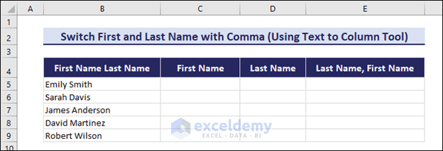
3. Using Convert Text to Columns Wizard and Excel CONCAT Function to Switch First and Last Name in Excel with Comma
Splitting First Name and Last Names into two parts using Convert Text to Columns Wizard and then joining those parts with commas using Excel CONCAT functions, you can switch first name and last name in Excel with commas.
Excel’s Convert Text to Columns Wizard feature splits the content of one cell into multiple cells using the delimiters (comma, space, semicolon, etc.) you choose.
In this method, we shall use the Convert Text to Columns Wizard to split column B into columns C and D. It will separate the first and last names. Then we shall use the CONCAT function in column E to join the last name and first name with a comma and a space.
This is the dataset I am going use.
Follow the steps:
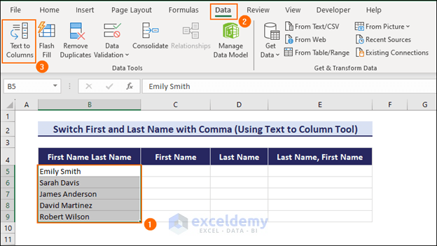
Step 1: Select the range B5:B9.
=> Click on the Data tab => Data Tools group of commands => Click on the Text to Columns command.
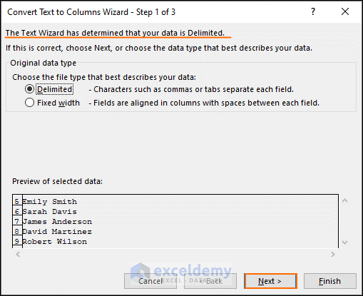
Step 2: The Convert Text to Columns Wizard will appear. It is Step 1 of 3. The text wizard has detected correctly that our data is Delimited. So, click on Next.
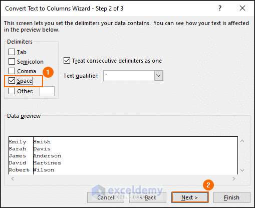
Step 3: In Step 2 of 3, check the option Space under the field Delimiters => Click on the Next option.
Step 4: In the final step, select the General option under the Column data format field => Select the cell location (C5, it is the first cell of the First Name column) where you want to get the values under the Destination field => Click on Finish.
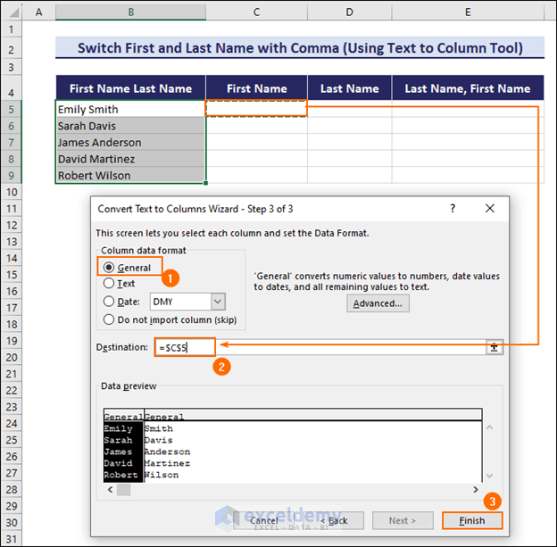
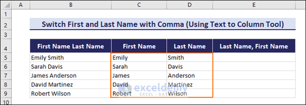
When you click on Finish, the text data of column B is split into columns C and D perfectly.
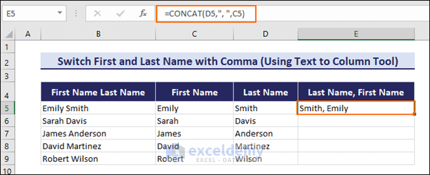
Now, we shall use the CONCAT function to join the Last Name and First Name columns with a comma and a space.
Step 5: Write this formula in cell E5 and hit the Enter button.
=CONCAT(D5,”,”,C5)You will get the first and last names switched with a comma.
Step 6: Use the AutoFill feature to fill the formula for the rest of the cells.
Read More: How to Reverse Names in Excel
4. Using Power Query to Switch First and Last Name in Excel with Comma
In this section, you will learn how to switch first name and last name in Excel using Excel’s Power Query tool.
If you have to switch first and last names with comma quite often, it wouldn’t be a good choice to use Flash Fill or formulas each time. You can use the Power Query to switch first and last name with comma. Then you can use the same query multiple times with various datasets.
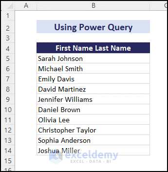
We shall use the following dataset. It contains 10 first and last names.
Follow the steps:
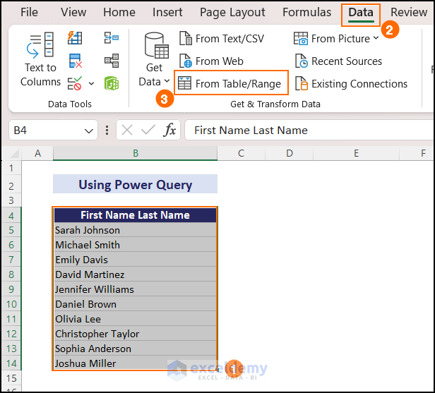
Step 1: Select the dataset including the header => Click on the Data tab => Get & Transform Data group of commands => Select From Table/Range option.
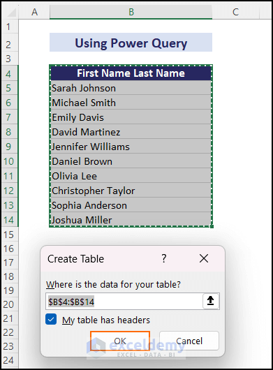
Step 2: You will get a Create Table dialog box. Under where is the data for your table? field, the selected data range is showing. As you have selected the dataset including the header, My table has headers option is checked automatically.
=>Press the OK button.
After clicking OK, you will get a table in Power Query Editor created with the selected range.
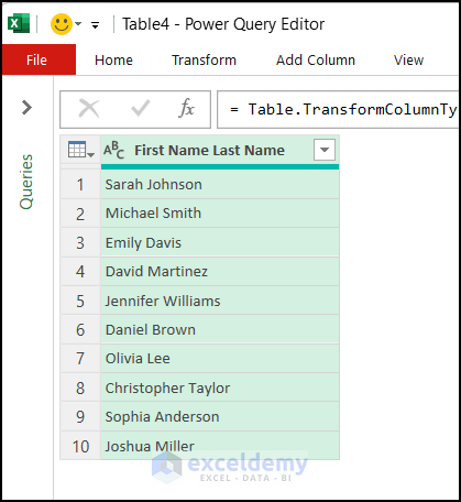
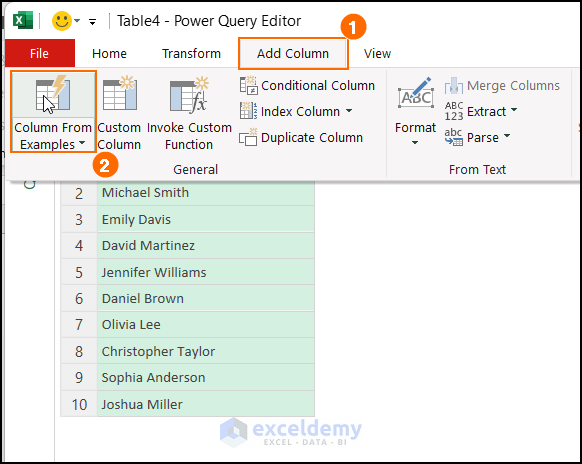
Step 3: In Power Query Editor, click on the Add Column tab =>General group of commands, select the Column From Examples option.
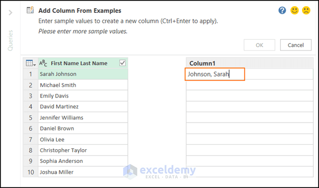
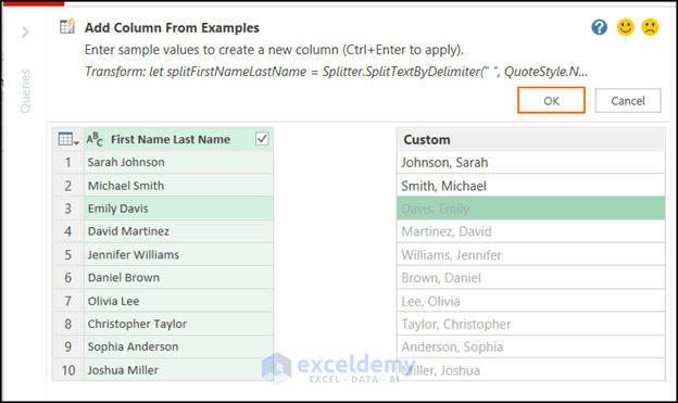
Step 4: A new column named Column1 is added. You have to set examples in this column so that the Power Query can detect the pattern.
=> Write Johnson, Sarah in the first row of the column.
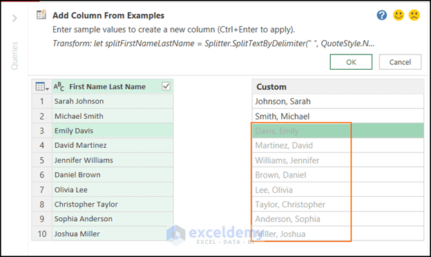
Step 5: Give another example in the second row “Smith, Michael” and press Enter.
After pressing Enter, the other cells will show suggestions. The suggestions are correct so you don’t have to provide any more examples.
Note: Check the suggestions properly. If it doesn’t match your requirements, you have to give more examples. Keep providing examples until it matches your pattern properly.
Step 6: Press the OK button or just use the keyboard shortcut Ctrl+Enter to apply the suggested values.
Note: It is not mandatory to provide examples from the first row of the column. You can start providing the examples from any row of the Custom Column.
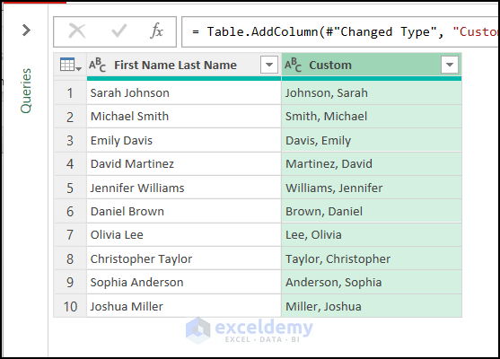
Thus, you will get the first and last names switched with commas.
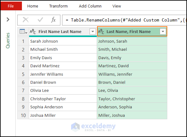
Step 7: Double-click on the column header and rename it according to your preference.
Step 8: Right-click on the first column =>Select Remove.
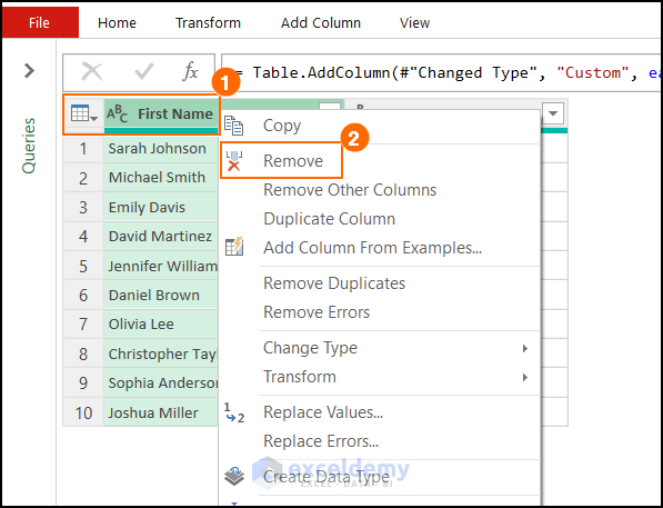
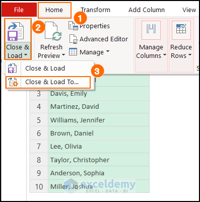
Step 9: The first column is removed. To load the Last Name, First Name column in the Excel worksheet,
=>Click on the Home tab => Select Close & Load dropdown => Click on the Close & Load To option.
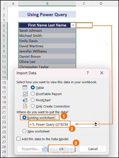
Step 10: The Import Data dialog box will appear. The Table option is selected by default.
=>Select Existing Worksheet.
=>Select the cell where you want to load the table.
=>Click on the OK button.
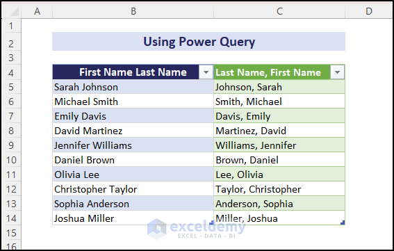
As a result, you will get the switched first and last names in your worksheet.
5. Using Power Pivot
In this section, we shall use the Power Pivot add-in of Excel to switch first and last name in Excel with comma. Power Pivot is a powerful data analysis tool. It is available as an add-in for Microsoft Excel.
In Power Pivot, we shall add a calculated column where we will use DAX (Data Analysis Expressions) formula to switch the first and last name with comma. Later we shall present that column with a PivotTable.
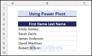
We shall use the same dataset. Our goal is to switch the first and last names of column B with commas.
Follow the steps:
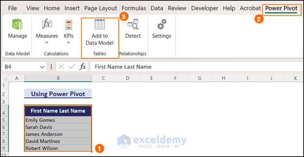
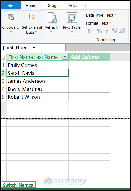
Step 1: Select the entire range where you have your dataset =>Click on the Power Pivot tab =>Select the Add to Data Model option.
Note: In case, you don’t have the Power Pivot tab, enable the Power Pivot add-in first.
Step 2: Create Table dialog box will appear. As we have selected the range before, it is showing already. Press the OK button.
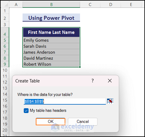
You will see the selected column in Power Pivot window.
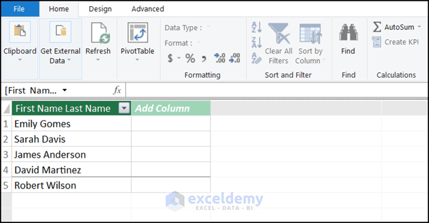
Step 3: To rename the table name, Double-click on the table name which is set as Table1 by default.
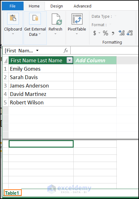
Step 4: Rename this table according to your choice. Try to give a relevant name.
We renamed it as Switch_Names.
Step 5: Click on Add Column.
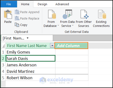
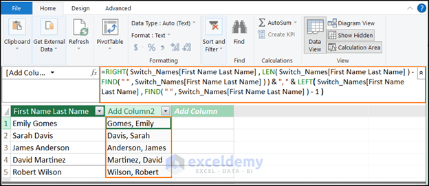
Step 6: A new column is added. Write this DAX formula in the formula bar of the newly added column and press Enter.
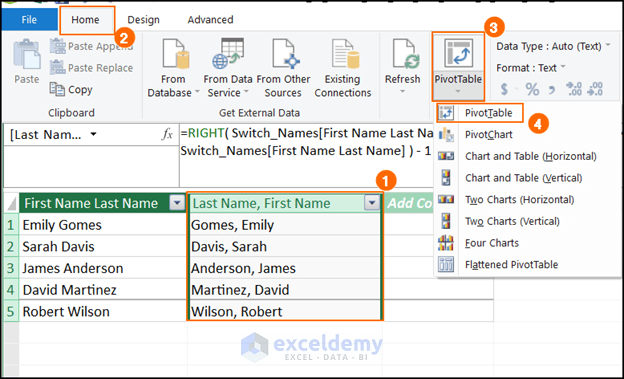
=RIGHT( Switch_Names[First Name Last Name] , LEN( Switch_Names[First Name Last Name] ) - FIND( " " , Switch_Names[First Name Last Name] ) ) & ", " & LEFT( Switch_Names[First Name Last Name] , FIND( " " , Switch_Names[First Name Last Name] ) - 1 )Therefore, you will get the new calculated column. Here, the first and last names are switched with commas.
Note: This formula is similar to the formula we used in Excel worksheet using text functions. Power Pivot has a formula language known as DAX. The difference is Excel formulas work for a single cell at a time. But DAX formula works for the entire column.
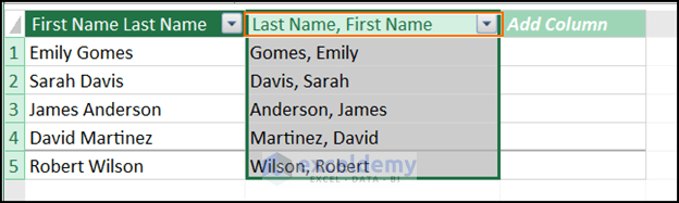
Step 7: Double-click on the column header and rename it. We have renamed it as Last Name, First Name.
Step 8: Select the calculated column =>Click on the Home tab =>Select the PivotTable dropdown =>Select the PivotTable option.
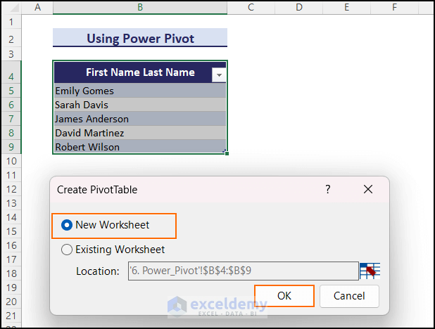
Step 9: The Create PivotTable dialog box will appear. The option New worksheet is selected by default. So, press OK.
You will see, a new Excel worksheet is opened and you have to choose the fields from the PivotTable field list.

Step 10: Choose the field Last Name, First Name from the Switch_Names table.
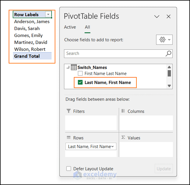
We have created the PivotTable where we get the first and last names switched with commas.
6. Applying VBA Code to Switch First and Last Name in Excel with Comma
In this section, you will learn applying VBA code to switch first and last name in Excel with comma.
If you have to switch first and last names with commas multiple times in a workbook, creating a VBA code for this action is the best solution. You can use this VBA code for multiple datasets. It will save time and effort.
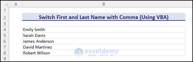
We shall use the following dataset to run the VBA code.
Follow the steps:
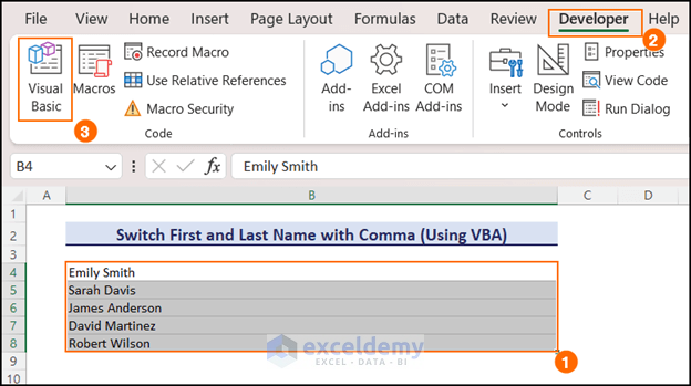
Step 1: To write any VBA code, you must launch the VBA editor first. To do that,
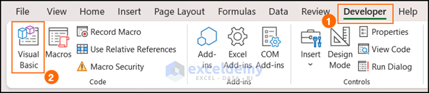
=>Click on the Developer tab from Excel Ribbon. If you don’t have the Developer tab in Excel Ribbon, you have to enable it from Excel Options.
=>Afterward, select the Visual Basic option.
Note: Alternatively, you can press Alt+F11 to open the VBA editor.
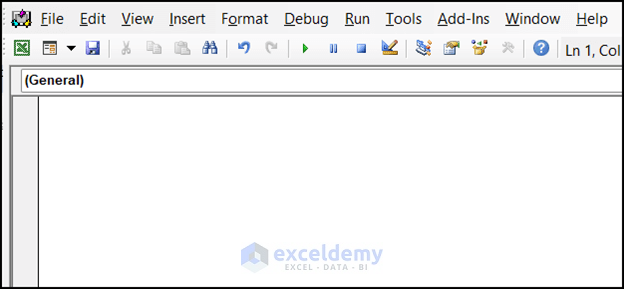
 Step 2: After clicking on Visual Basic, Excel will lead you to the VBA Editor Window. In this window, you can write your VBA code.
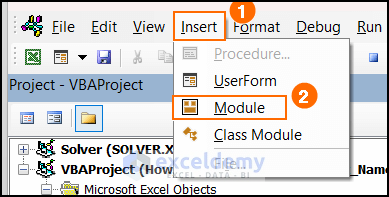
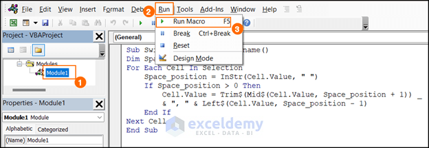
Step 3: Now, select Insert => Click on Module.
Step 4: You have inserted a new module. Now, copy this code to the module and save the sub procedure.
Sub Switch_first_and_last_name()
Dim Space_position As Long
    For Each Cell In Selection
    Space_position = InStr(Cell.Value, " ")
        If Space_position > 0 Then
            Cell.Value = Trim$(Mid$(Cell.Value, Space_position + 1)) _
            & ", " & Left$(Cell.Value, Space_position - 1)
        End If
    Next Cell
End Sub
VBA code to switch first and last name in Excel with comma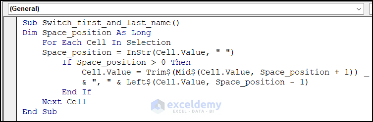
Note: Don’t forget to save your workbook as a Micro-Enabled Workbook.
Step 5: Go back to the Excel worksheet and select the range for which you want to switch first and last name with comma.
=>Select the Developer tab => Code group of commands => Select the Visual Basic option.
Step 6: Click on Run => Run Macro or just use the keyboard shortcut F5 to run the code.
Step 7: Right after running the code the first and last names are switched with comma. Go to the Excek worksheet and you will notice the changes. The first and last names are switched with commas successfully.
Note: If you run the VBA code once, you cannot undo this action. So it is a good idea to store the backup copy of the original dataset before running the VBA macro. In case, you need the original version you can get it.
Note: You can save this VBA code in your personal macro enabled workbook. Then, add the macro to the quick access toolbar with a relevant icon. By doing this, you can use this code multiple times just by clicking on the macro icon from the quick access toolbar. It will definitely save your time and effort.
Download Practice Workbook
Conclusion
In this Excel tutorial, you have learned how to switch first and last name in Excel with comma. For example, we showed to reverse Emily Smith to Smith, Emily. You can switch first and last name with comma in several ways. The easiest method is using the Flash Fill feature. But as it is not a dynamic fix, we showed other ways like using formulas, using Convert Text to Columns Wizard, using Power Query, using Power Pivot, and applying Excel VBA code. We hope, from this tutorial, you have learned how to switch first and last name in Excel with comma.
Related Readings
- How to Reverse a String in Excel
- How to Use Excel VBA to Reverse String
- How to Reverse a Number in Excel
- How to Paste in Reverse Order in Excel
- How to Reverse Rows in Excel
<< Go Back to Excel Reverse Order | Sort in Excel | Learn Excel
Get FREE Advanced Excel Exercises with Solutions!

Hiya – great article – could you help with the following please ?
My list of names isn’t consistent in terms of number of forenames as I have people from the UK and from Singapore in the list I am manipulating.
For the UK – the majority are surname,forename so I can use your method above.
For Singapore I have:
Surname, forename2 forename1
or
Surname, forename2 forename3 forename1
(only one comma in the string)
I would like this to be
Forename1 Forename2 (forename3) Surname
Is this possibe ?
Many thanks in advance for your help
Hi, GEOFF BARTLETT! We appreciate your thoughtful query.
Workaround 1:
For your first problem (Surname, forename2 forename1), you can use the formula below:
=SUBSTITUTE((RIGHT($B7,LEN($B7)-FIND("^",SUBSTITUTE($B7," ","^",LEN($B7)-LEN(SUBSTITUTE($B7," ",""))))))&" "&(MID($B7,SEARCH(" ",$B7)+1,SEARCH(" ",$B7,SEARCH(" ",$B7)+1)-(SEARCH(" ",$B7)+1)))&" "&(LEFT($B7,SEARCH(" ",$B7)-1)),",", "")And, for your second problem (Surname, forename2 forename3 forename1) you can use the formula below:
=SUBSTITUTE((RIGHT($B5,LEN($B5)-FIND("^",SUBSTITUTE($B5," ","^",LEN($B5)-LEN(SUBSTITUTE($B5," ",""))))))&" "&(MID($B5,SEARCH(" ",$B5)+1,SEARCH(" ",$B5,SEARCH(" ",$B5)+1)-(SEARCH(" ",$B5)+1)))&" "&"("&(MID($B5,SEARCH(" ",$B5,SEARCH(" ",$B5,1)+1)+1,SEARCH(" ",$B5,SEARCH(" ",$B5,SEARCH(" ",$B5,1)+1)+1)-(SEARCH(" ",$B5,SEARCH(" ",$B5,1)+1)+1)))&")"&" "&(LEFT($B5,SEARCH(" ",$B5)-1)),",", "")Workaround 2:

Besides, another workflow you can use in this regard. That is:
Step 1: Use the Text to Columns tool from the Data tab for splitting every name.
https://www.exceldemy.com/text-to-columns-excel/
Step 2: Sort them according to your desired sequence. Use a helper row for that. Use and finally >>

Last Step: Use the CONCATENATE function to combine them in a cell.

https://www.exceldemy.com/excel-concatenate-function/
Regards,
Tanjim Reza
Hello are you presentto help
Wish to make John Smith > Smith J
Thank you.
Hi, JUSTIN!
Thank you for your query.
You can accomplish your desired result by using the formula below:
Regards,
Tanjim Reza