While working with Excel, there are situations when you are comparing data between two or more ranges and calculating with multiple criteria. The SUMPRODUCT function is an extremely resourceful function for these purposes. It has the unique ability to handle arrays in smart and elegant ways. Often, we need to use this function to compare between columns with given criteria and to find the result. Today in this article, we will discuss some methods of using the SUMPRODUCT function with criteria.
Excel SUMPRODUCT Function: Overview
Technically, the “SUMPRODUCT” function remits the summation of the values of corresponding arrays or ranges.
⇒ Syntax
The syntax of the “SUMPRODUCT” function is simple and direct.
=SUMPRODUCT(array1, [array2], [array3], …)
⇒ Argument
| Argument | Required/Optional | Explanation |
|---|---|---|
| array1 | Required | The first input to an array, whose elements you want to divide and afterward add. |
| [array2], [array3] | Optional | Array parameters with elements you want to multiply and add, ranging from 2 to 255. |
Note: One of the amazing features of the SUMPRODUCT function is it can handle single or multiple criteria remarkably well. Let’s discuss some of the SUMPRODUCT with criteria functions.
1. Applying SUMPRODUCT with a Single Criterion to Lookup Value
We can apply the SUMPRODUCT function with criteria with or without the double unary operator.
1.1. Using Double Unary Operator
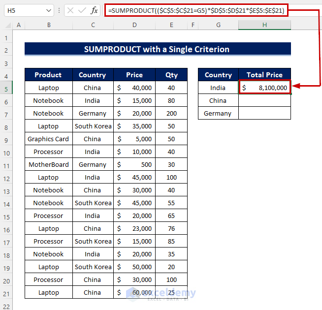
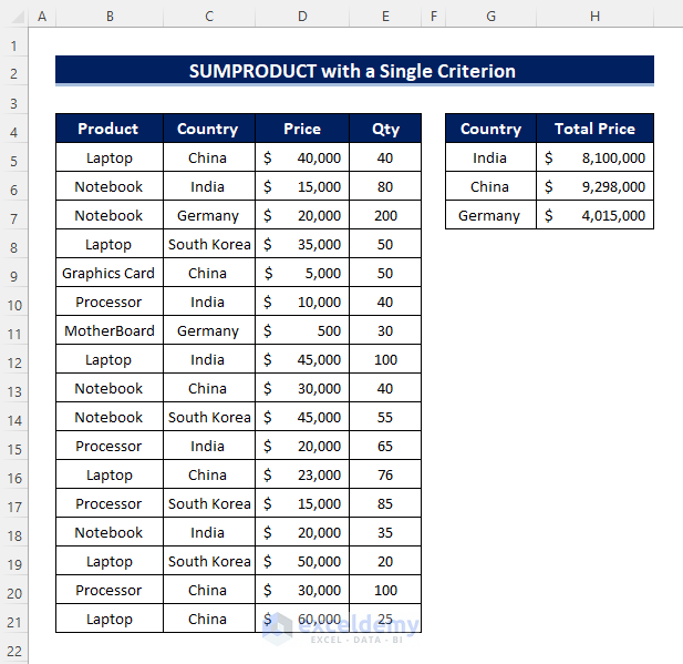
A smart way to apply the SUMPRODUCT function is to insert the criteria within the function as an array using “Double unary operator (–)” to convert the “TRUE” or “FALSE” into “1” or “0”. In the following example, some “Product” names are given with their “Country”, “Qty”, and “Price”. We will find the total price for countries “India”, “China”, and “Germany”.
Let’s follow the procedures to use the SUMPRODUCT function with single criteria in Excel.
STEPS:
- Firstly, create a table for these countries anywhere in the worksheet where you want to get the result.
- Secondly, select the cell where you want to put the formula of the SUMPRODUCT function.
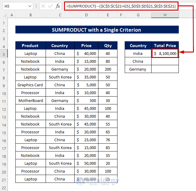
- Thirdly, insert the formula into that cell. We apply the function with the “Double Unary Operator (–)”.
=SUMPRODUCT(--($C$5:$C$21=G5),$D$5:$D$21,$E$5:$E$21)- Then, press the Enter key. We have got the total price for “India”.
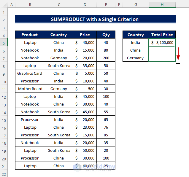
- Drag the Fill Handle icon down to duplicate the formula over the range. Or, to AutoFill the range, double-click on the plus (+) symbol.
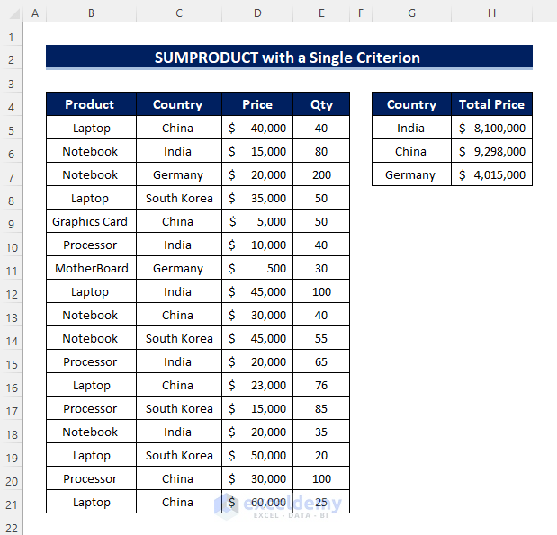
- Finally, we can see the results for India, China, and Germany.
🔎 How Does the Formula Work?
- Array1 is –($C$5:$C$21=G5) G5 is “India”. The double unary operator will convert the results from $C$4:$C$20 into “1” and “0”.
- [Array2] is $D$5:$D$21, which range we first multiply and then add.
- [Array3] is $E$5:$E$21, also this range we multiply and then add.
We will use the “Absolute Cell References” to “BLOCK” the cells.
Read More: How to Use SUMPRODUCT Function with Multiple Columns in Excel
1.2. Excluding Double Unary Operator
We can solve the previous example without using the double unary operator. Let’s see the instructions for this.
STEPS:
- We will use the same example to get the same result. Now, in Cell “H5” apply the SUMPRODUCT function. Insert the values into the formula and the formula is like this.
=SUMPRODUCT(($C$5:$C$21=G5)*$D$5:$D$21*$E$5:$E$21)
- Further, hit the Enter key to show the outcome.
- To copy the formula over the range, drag the Fill Handle symbol downward. Alternatively, you can double-click the addition (+) sign to AutoFill the range.
- Similarly, we can get the result.
2. Using SUMPRODUCT with Multiple Criteria for Different Columns
We can apply the SUMPRODUCT function with multiple criteria with or without the double unary operator. Let’s learn!
2.1. Using Double Unary Operator
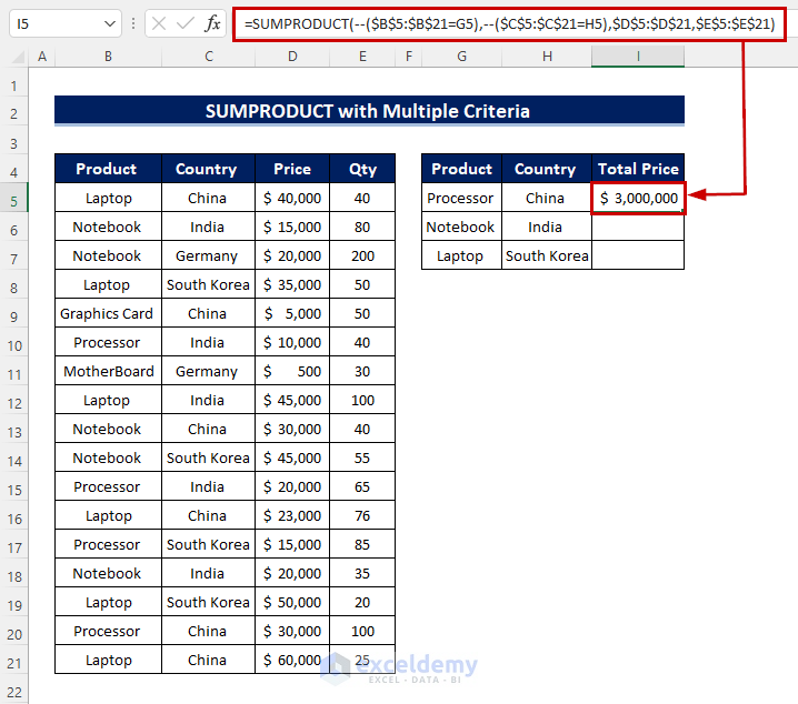
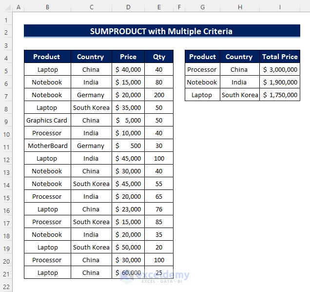
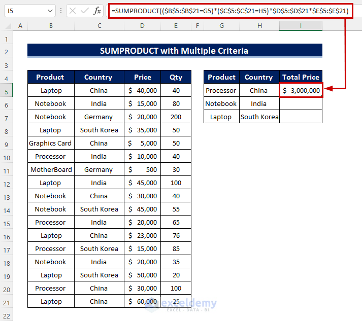
In this case, we will use the “Double Unary Operator (–)” to convert the array results into “1” or “0”. Consider the same table that we used before. Now we will find the result using multiple criteria. We will find the “Total Price” for “processor” of the country “China”, “Notebook” of “India” and “Laptop” of “South Korea”. Using these criteria we will derive the result.
STEPS:
- In the beginning, select a cell adjacent to the first book and enter the formula.
=SUMPRODUCT(--($B$5:$B$21=G5),--($C$5:$C$21=H5),$D$5:$D$21,$E$5:$E$21)- Press the Enter key on your keyboard once more.
- Likewise, in the previous examples, drag the Fill Handle icon down to duplicate the formula over the range. Or, to AutoFill the range, double-click on the plus (+) symbol.
- Finally, you will get your results.
2.2. Excluding Double Unary Operator
Here we will apply the same multiple criteria using the basic SUMPRODUCT function.
STEPS:
- In cell I5, apply the function. Insert the criteria and the formula looks like this.
=SUMPRODUCT(($B$5:$B$21=G5)*($C$5:$C$21=H5)*$D$5:$D$21*$E$5:$E$21)- Hit Enter to see the result.
- After that, drag the Fill Handle icon to copy the formula over the range. Or, double-click on the plus (+) sign. This also duplicates the formula.
- Finally, you can see the outcome.
Read More: How to Use SUMPRODUCT to Lookup Multiple Criteria in Excel
3. Inserting SUMPRODUCT Function with OR Logic
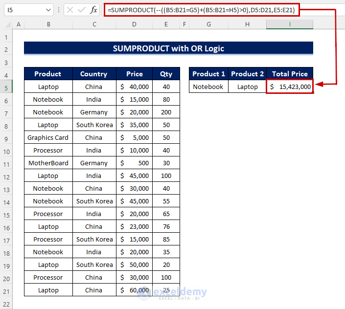
We can add OR logic to our formula to make the SUMPRODUCT function with criteria more dynamic. Consider the situation where we need to find out the total price for “Notebook” and “Laptop”.
STEPS:
- Firstly, create a table anywhere in the worksheet where you want to get the result.
- Then, select the cell and insert the following formula there.
=SUMPRODUCT(--((B5:B21=G5)+(B5:B21=H5)>0),D5:D21,E5:E21)- Further, hit the Enter key to see the outcome.
Related Content: Excel SUMPRODUCT Function Based on Date Range
4. Applying SUMPRODUCT with Multiple AND/OR Criteria
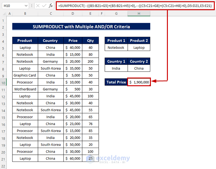
In this method, we will apply the SUMPRODUCT function with criteria using both “AND”, “OR” logic. This time we have to add more criteria to our function. We will retrieve the “Total Price” for the product “Notebook”, “Laptop” of the country “India”, “China”.
STEPS:
- To begin with, select the second cell H10, and put the formula into that selected cell.
=SUMPRODUCT(--((B5:B21=G5)+(B5:B21=H5)>0),--((C5:C21=G8)+(C5:C21=H8)>0),D5:D21,E5:E21)- Then, press the Enter key to see the outcome.
🔎 How Does the Formula Work?
- 1 is –((B5:B21=G5)+(B5:B21=H5)>0),–((C5:C21=G8)+(C5:C21=H8)>0). Here B5:B21 is the “Product” Column, G5 and H5 are “Notebook” and “Laptop”. Similarly, C5:C21 is the “Country” column, and G6 and H6 are “India” and “China”.
- [Array2] is D5:D21.
- [Array3] is E5:E21.
Read More: How to Use SUMPRODUCT IF in Excel
5. Using SUMPRODUCT with Multiple Criteria for Rows and Columns
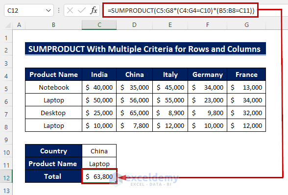
The “SUMPRODUCT” function shows its true diversity when we use this function for both columns and rows. Let’s see how. In the following example, we can see the price of some “Products” from the country “India”, “China”, “Italy”, “Germany”, “France”.
STEPS:
- Firstly, select the cell where we want to put the result.
- Then, insert the formula into that cell.
=SUMPRODUCT(C5:G8*(C4:G4=C10)*(B5:B8=C11))- Finally, press Enter key from the keyboard.
Read More: Excel SUMPRODUCT with Multiple Criteria in Same Column
Things to Remember
✅ The “SUMPRODUCT” function treats non-numeric values as zeros. If you have any non-numeric values in your formula the answer will be “0”.
✅ Arrays in the SUMPRODUCT formula must have the same number of rows and columns. If not, you get the #VALUE! Error.
✅ The “SUMPRODUCT” function does not support wildcard characters.
Download Practice Workbook
Download this practice sheet to practice the task while you are reading this article.
Conclusion
The SUMPRODUCT function is one of the most diversified functions in Excel. In this article, we covered the SUMPRODUCT function with single or multiple criteria. We hope that this article proves useful to you. If you have any confusion or suggestions, you are welcome to comment.
Related Articles
- SUMPRODUCT Across Multiple Sheets in Excel
- SUMPRODUCT for Counting with Multiple Criteria in Excel
- [Solved] SUMPRODUCT with Multiple Criteria Not Working in Excel
<< Go Back to Excel SUMPRODUCT Function | Excel Functions | Learn Excel
Get FREE Advanced Excel Exercises with Solutions!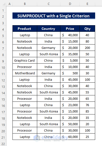



I believe there’s an error in “5) SUMPRODUCT with Multiple Criteria for Rows and Columns “: the answer calcualated by SUMPRODUCT()($63,800) should actually be only $56,000 (the intersection of Laptop and China).
Dear FLEET,
Thank you for your response.
The answer for the intersection of “Laptop” and “China” will be “$63,800”.
The SUMPRODUCT function returns the sum of an array from an argument. With the intersection between “China” and Laptop” within the cell range we got two outputs which are “$56,000” and “$7,800”. Thus summing the total value with the SUMPRODUCT function stands to “$63,800”.
You can check the screenshot below.
We have also attached a worksheet with our article. You can practice the formula there, too. Thanks!
Thanks for referring, I will check.
u made my day. i was struggling with multiple selections!… thanks a lot
Hello, KRISHNAN V! Thanks for your feedback. Hope you’ll find our other articles useful as well when needed for your works!
How can I use the SUMPRODUCT for adding sums from different columns that are under the same category in a drop-down list? For this example, I split up my expenses for each pay check and then I categorize each expense by an “expense type”. I want each expense for each expense type to be added together to a separate table that I will then use those sums to create a pie chart. For example, I have a pay check on 9/15 where my Lifestyle expense = $200 and a pay check on 9/30 where the Lifestyle expense= $350. In the other table, I want to be able to add the sum of $200+$350. Can SUMPRODUCT help me with this? I have been struggling a lot to figure this out! I can provide a screen shot of the excel chart if needed.
Hello FELICIA SANTOS,
I hope you are doing well! Here, I have created a dataset as you have described and calculated the total amount spent per category.
>> Here, you have to insert the name of the category in cell F5.
>> Then, insert the following formula into cell G5:
=SUMPRODUCT(D3:D10*(C3:C10=F5))Thus, you will get the sum of the amount as per the selected category.
I hope, your problem will be solved in this way. You can share more problems in an email at [email protected]
Hi,
What if I want to sum Notebook from India up to France (Result = $ 167,000.00)
or
Product : Notebook
From : China
To : Germany
Result = $114,000
From & To in dropdown list
Hello DRIN,
Thanks for your comment.
If you want to sum Notebook from India up to France and use drop-down for the countries, then use the following formula in cell C13:
=SUM(INDEX($B$5:$G$8,MATCH(C10,$B$5:$B$8,0),MATCH(C11,$C$4:$G$4,0)+1):INDEX($B$5:$G$8,MATCH(C10,$B$5:$B$8,0),MATCH(C12,$C$4:$G$4,0)+1))
It’ll give the desired result.
Change the countries to China and Germany from the drop-down and the total value will be updated.
If you have other queries let me know in the comment.
Regards,
Sajid Ahmed
Exceldemy
very help information. I managed to resolve my equation for sumproduct.
Thanks a lot
KS
Hello,
You are most welcome.
Regards
ExcelDemy