Creating a sprint burndown chart is now an essential part of the inventory management system. Sprint burndown chart aids the team in determining how many tasks are still in the bucket and showing how long each task takes to complete. This makes it simpler for stakeholders and other participants to estimate when the sprint’s objectives will be met. So, this article will discuss how to create a sprint burndown chart in Excel.
What Is a Sprint Burndown Chart?
The sprint burndown chart is a simple tool that allows users to see how close they are to meeting the sprint goal by the end of the sprint. Burndown charts, which show the pattern of work remaining over time in a sprint, are popular in scrums. The Sprint Backlog serves as the initial source of data for a burndown, with the amount of work still to be done being monitored on the vertical axis and the duration (days of a sprint) being tracked on the horizontal axis.
Sometimes people find it hard to make the difference between a product burndown chart and a sprint burndown chart. To ease your confusion, a product burndown chart displays the amount of work that needs to be done on the overall project, whereas a sprint burndown chart displays the amount of work that needs to be done on a specific rotation.
Sprint Burndown Chart in Excel: 5 Easy Steps to Create
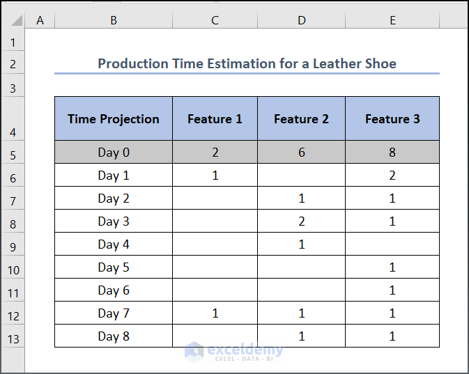
Let’s assume we have a dataset, namely “Production Time Estimation for a Leather Shoe”. You can use any dataset suitable for you.
Here, we have used the Microsoft Excel 365 version; you may use any other version according to your convenience.
Step 1: Prepare the Dataset
The very first step to creating a sprint burndown chart is to prepare the dataset with the additional information. Look at the image we have attached below.
- Here, we want to create a sprint burndown chart for leather shoes. The bulk production of a specific shoe requires a considerable amount of time as there are multiple features that need to be added one by one.
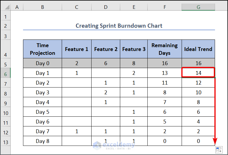
- We consider a specific type of shoe that comprises three distinguishable features. Features 1, 2, and 3 all demand 2, 6, and 8 days respectively. Thus, we need 16 working days to complete the whole process.
- As you can see from the given figure below, we distributed those allocated days into a time span of 8 days.
Read More: How to Create Risk Burndown Chart in Excel
Step 2: Calculate Remaining Days
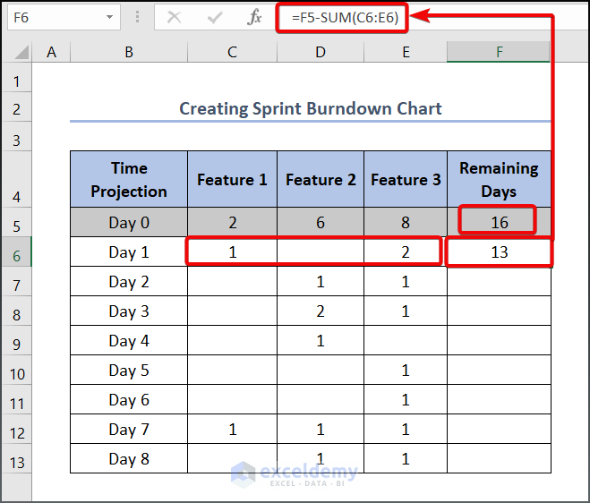
The second step of the sprint burndown chart is to calculate the remaining days. These days will assist you in determining how much time you have left on your inventory to complete your manufacturing process. We’ll use the data to create a sprint burndown chart later.
- Write down the following formula in cell F6.
=F5-SUM(C6:E6)
- Subsequently, press Enter and see the output given below.
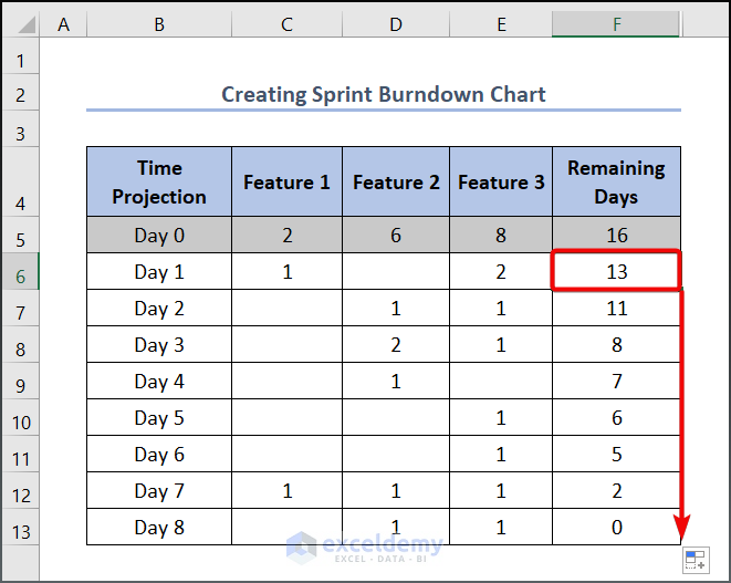
- Drag the Fill Handle tool to get the other values.
Step 3: Determine Ideal Trend
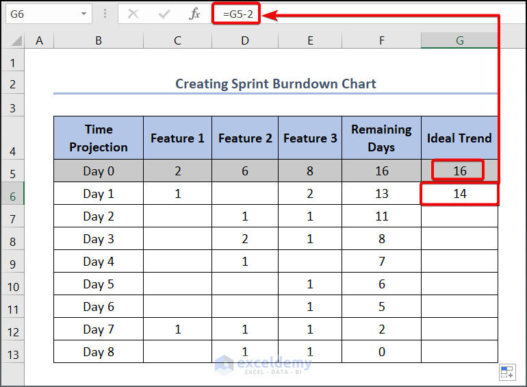
As you know, all physical phenomena are compared with an ideal scenario to fully understand their practical behavior and thus analyze the deviation later. So, we will now create an ideal trend that will tell you the number of days remaining in the process in an ideal condition.
- As we are allocated 16 working days to complete the process and the time span is 8, we will decrease 2 working days on each day.
- To get the Ideal Trend, write the following formula in the G6 cell.
=G5-2
- Press the Enter button to see the output.
- To get the other value drag the Fill Handle tool below.
Step 4: Create Sprint Burndown Chart
As you know, using Excel charts, you can visualize your workbook data to see its trends. Excel charts can also be used to display comparisons. So, it’s time to create the sprint burndown chart in Excel. Follow the process, which we are going to describe below, to accomplish the task.
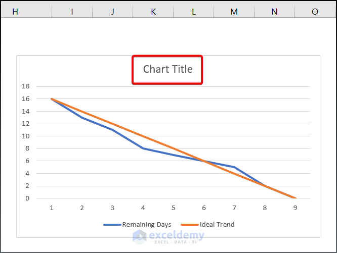
- Select the data of F4:G13 cell range then move onto Insert >> Line or Area Chart.

- Then click on the Line chart.

- Now see the output which has been given below.

Read More: How to Create Budget Burndown Chart in Excel
Step 5: Format the Sprint Burndown Chart
We have calculated the remaining days, and the ideal trend, and created a sprint burndown chart so far. Now we need to label the axis with an appropriate title so that anyone can easily interpret the idea of the chart.
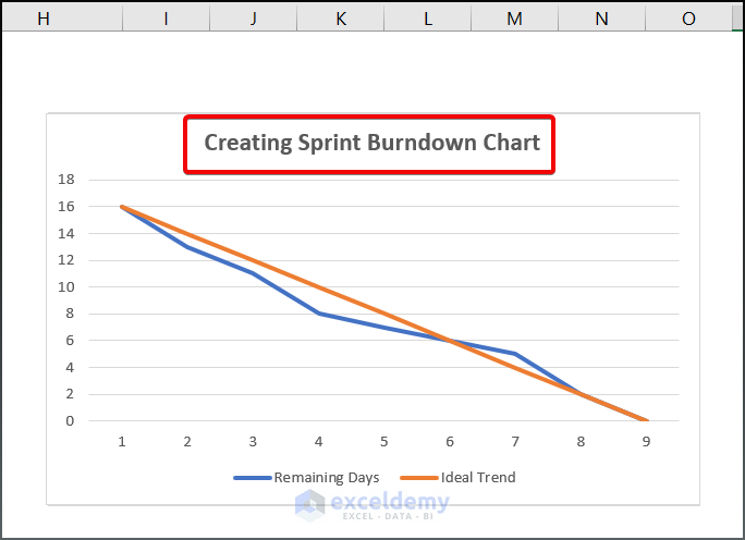
- First, double-click on the Chart Title box and write the title as Creating Sprint Burndown Chart.
- Press Enter and see the output given below.
- Now it is time to label the title of the X-axis. To do so, select the chart and then click on the right button of the mouse. Subsequently, click on Select Data…

- Select data from B5 to B13
- Press OK afterward.

- Thus, another dialog box will appear. Press the OK button selected by the red box.

- That’s it. Our sprint burndown chart is ready to present. Now see the output as given below.

Read More: How to Create a Burn-up Chart in Excel
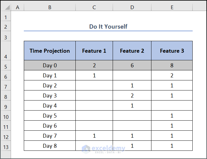
Practice Section
We have provided a Practice section on the right side of each sheet, so you can practice yourself. Please make sure to do it yourself.
Download Practice Workbook
You can download and practice the dataset we have used to prepare this article.
Conclusion
We hope you got an overall idea about creating a sprint burndown chart in Excel. If you have any queries regarding the process or anything related to this topic, feel free to make a comment below. We will get back to you soon.
<< Go Back to Burndown Chart in Excel | Excel Charts | Learn Excel
Get FREE Advanced Excel Exercises with Solutions!
