How to Create a Budget Burndown Chart in Excel – 3 Steps

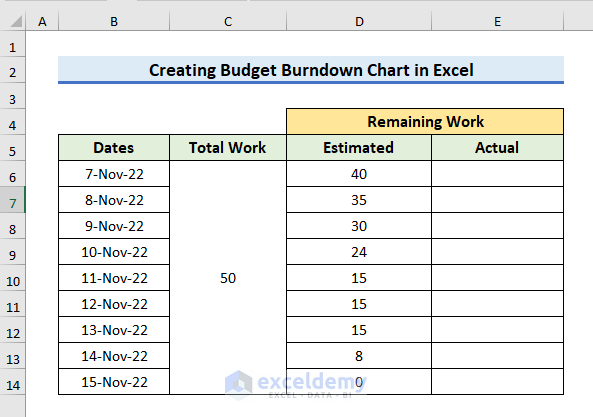
STEP 1 – Prepare a Dataset

This is the sample dataset. It showcases Total Work, Estimated Progress, and Dates.

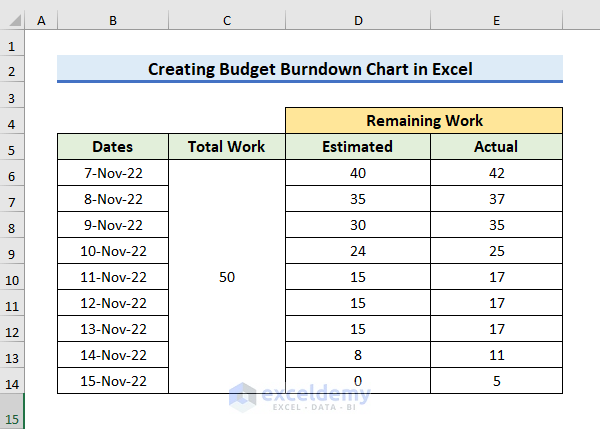
STEP 2 – Enter the Actual Task Progress in Dataset

• Enter the value of the remaining task at the end of each day in Column E.

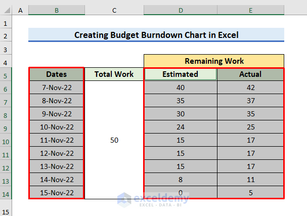
STEP 3 – Create a Budget Burndown Chart in Excel

• Select the Date, Estimated, and Actual Remaining Task columns.
• To select non-adjacent columns, select any column and hold Ctrl.
• Release Ctrl.

• Go to the Insert tab and select Insert Line in Charts.
• Select a type of line chart. Here, a 2-D line chart.

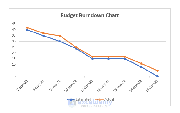
• The Budget Burndown chart is displayed.
• The Orange color indicates the pending percentage of tasks.
• The Blue color represents the remaining estimated tasks.

Final Output

• Rename the chart: Budget Burndown Chart.

Read More: How to Create a Burn-up Chart in Excel

Download Practice Workbook

To practice by yourself, download the following workbook.

Related Articles

• How to Create Sprint Burndown Chart in Excel
• How to Create a Burndown Chart in Excel

<< Go Back to Burndown Chart in Excel | Excel Charts | Learn Excel