Excel file sizes can get bigger if we have a large amount of data inside them. Decreasing the file size is one of the most important tasks whenever we want to share that file. There are numerous methods for reducing file sizes in Excel, but we will only concentrate on one of them. In this article, we will show you the quick steps to how to reduce Excel file size with the pivot table.
Pivot Table
The pivot table is one of the most useful tools in Microsoft Excel. This feature accumulates tons of data into an easy-to-read data table. This summarizes data into a report format. This feature saves a ton of time, and everyone who uses Excel as a daily driver should know how to work with a pivot table. There are four layout components to a pivot table: Filter, Column, Row, and Value. We can drag fields to these layout components to create a variety of pivot tables. When we create a pivot table, it creates a pivot cache, which remembers the source dataset. We can copy the pivot table into a new workbook and it will help us reduce the file size in Excel.
How to Reduce Excel File Size with Pivot Table: Step-by-Step Procedures
We will describe to you 3 easy steps to reduce file size with the pivot table in Excel.
Step 1: Setting Up Source Dataset
In the first step, we will prepare the source dataset.
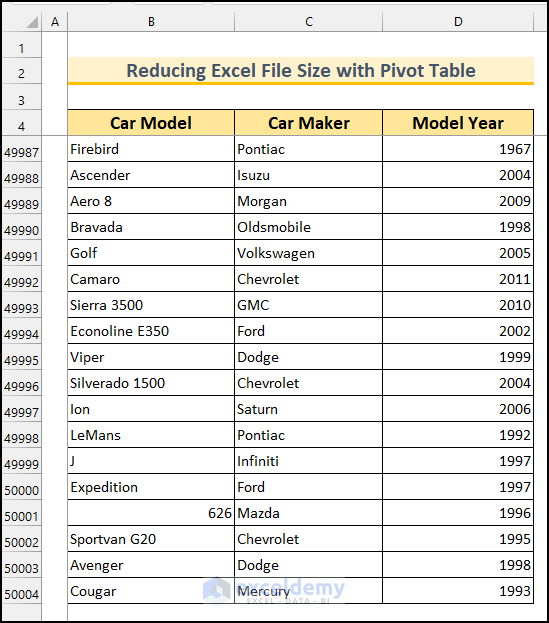
- There are 3 columns in our dataset consisting of Car Model, Car Maker, and Model Year. This represents data from car dealers in the USA.
- We have kept the row headings fixed up to row 4.
- We can see that there are 50,000 rows in this dataset.
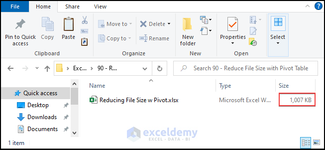
- After that, we Save and Close the file.
- We can see the file size is 1,007 KB.
Step 2: Inserting Pivot Table
In this step, we will insert a pivot table using the source dataset.
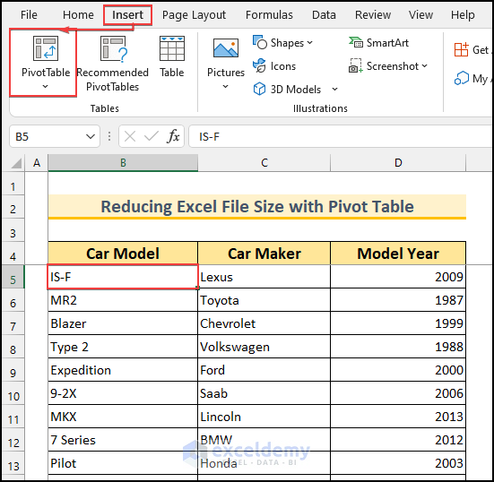
- Select anywhere inside the source dataset, we have selected cell B5.
- From the Insert tab → Select PivotTable.
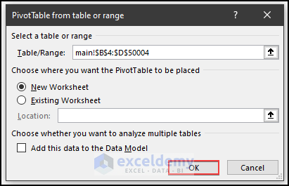
- The PivotTable from table or range dialog box will appear.
- Then, we kept every setting as it is and press OK.
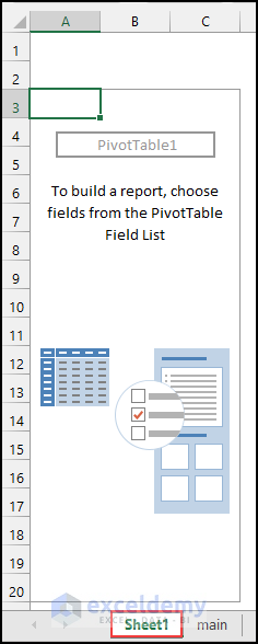
- A new worksheet named Sheet1 will be created on the workbook alongside the PivotTable1.
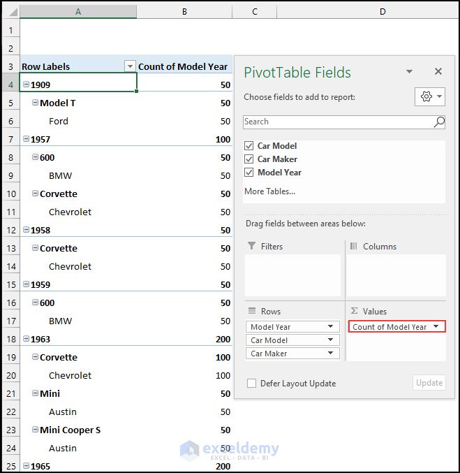
- Drag all three fields (Car Model, Car Maker, and Model Year) to the Rows area.
- Afterward, drag the Model Year field to the Values area.
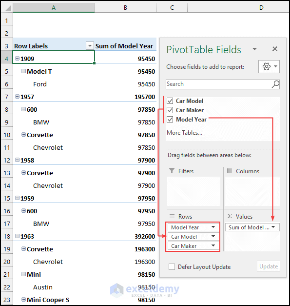
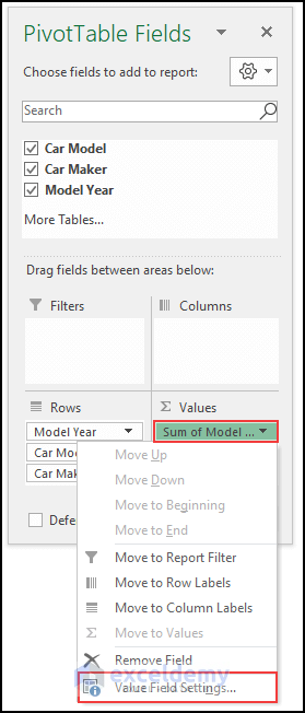
- In the Values area, Sum of Model Year will be shown. However, we want the Count of Model Year.
- In order to change that, click on it.
- Then, select Value Field Settings.
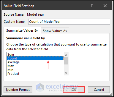
- The Value Field Settings box will pop up.
- Select Count and press OK.
- Afterward, the pivot table will look like this.
Step 3: Copying Pivot Table to New Workbook
In this last step, we will copy the pivot table to a new workbook and thus reduce the file size in Excel.
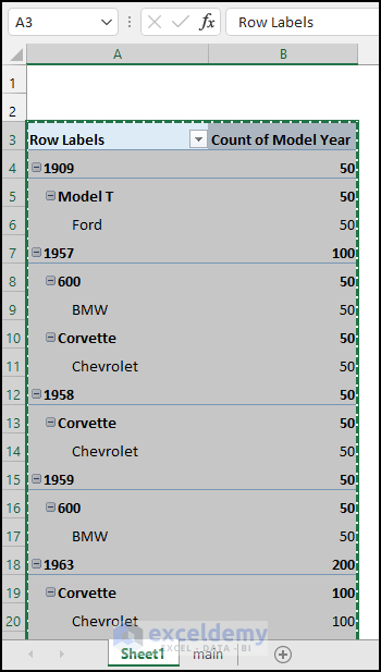
- Select the pivot table and press CTRL+C to copy it.
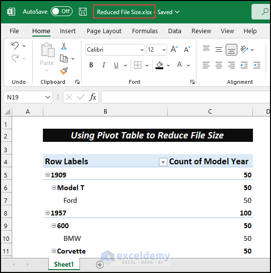
- Create a new workbook and press CTRL+V to paste the pivot table.
- Then, Save and Close the workbook.
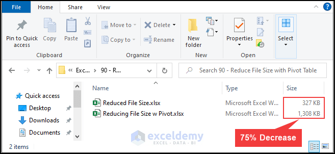
- We can see that the original file size increased a bit.
- Our new workbook is 327 KB in size compared to 1308 KB in the original file size. That is a whopping 75% reduction in file size. In other words, the reduced file size is only one-fourth of the original file size.
- Now, if we want to see the details of the dataset, then we can simply double-click on the Grand Total value.
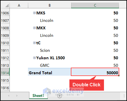
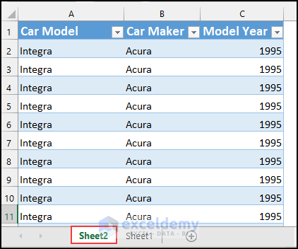
- A new worksheet called Sheet2 will be created to show the details of the data from the pivot table.
Read More: How to Reduce Excel File Size Without Deleting Data
Download Practice Workbook
Conclusion
We have demonstrated how to reduce the Excel file size with the pivot table in just three simple steps. If you face any problems regarding these methods or have any feedback for me, feel free to comment below. Moreover, you can visit our website for more Excel-related articles. Thanks for reading, and keep doing well!
Related Articles
- How to Zip an Excel File
- How to Compress Excel File for Email
- How to Reduce Excel File Size with Pictures
- How to Reduce Excel File Size with Macro
- How to Reduce Excel File Size Without Opening
- How to Reduce Excel File Size by Deleting Blank Rows
- How to Compress Excel File More than 100MB
- How to Compress Excel File to Smaller Size
- [Fixed!] Excel File Too Large for No Reason
- How to Determine What Is Causing Large Excel File Size
<< Go Back to Excel Reduce File Size | Excel Files | Learn Excel
Get FREE Advanced Excel Exercises with Solutions!
