To perform multiple tasks at once, we often use a nested formula in Excel. The nested formula saves time and cells in Excel. In this article, we’ll learn 3 easy ways to use a nested formula with the ROUND and AVERAGE functions in Excel with easy steps and proper illustrations.
Nested Formula with AVERAGE and ROUND Functions in Excel: 3 Easy Ways
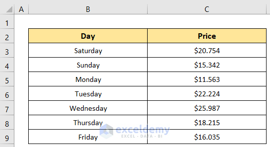
Let, the following dataset represent a product’s daily retail price for a particular week.
1. Using ROUND and AVERAGE Functions for a Nested Formula
First, we’ll nest a formula using the ROUND and AVERAGE functions to get a rounded average value. The ROUND function will round a decimal value according to the general mathematical rounding method. We can do it in the following two ways.
Find Average First Then Round
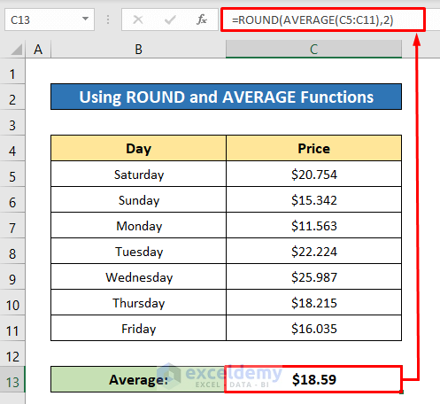
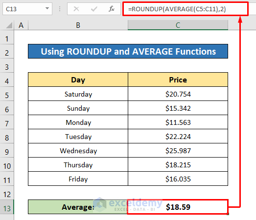
First, we can find the average value and then can round it. So we’ll have to use the AVERAGE function in the ROUND function as a nested formula. Here also we’ll keep two digits after the decimal.
Steps:
- Type the following formula in Cell C13–
=ROUND(AVERAGE(C5:C11),2)- Finally, just press the Enter button to get the result.
And see, we have got the same output as the previous method.
Formula Breakdown:
- AVERAGE(C5:C11)
Here, the AVERAGE function will return the average for the range C5:C11. And that will return as:
18.5885714285714 - ROUND(AVERAGE(C5:C11),2)
Later, the ROUND function will round the value according to specific digits. So the final nested formula will return as:
18.59
Round First Then Find Average
If we round every value first and then find the average for them that will give us the same output too. For that, I have added a new column- D to round the values.
Steps:
- In Cell D5, write the following formula-
=ROUND(C5,2)- Hit the Enter button to proceed.
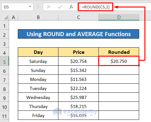
- Later, use the Fill Handle tool to copy the formula for the rest of the cells.

All the values are now rounded with two digits after the decimal. Let’s find the average now.
- Give input the following formula in Cell D13–
=AVERAGE(D5:D11)- Next, just press the Enter button to finish.

Read More: How to Create a Nested Formula in Excel
2. Applying ROUNDDOWN and AVERAGE Functions to Nest a Formula
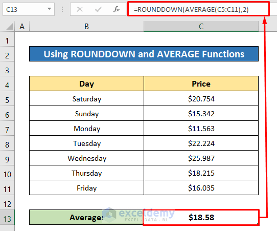
Previously, we saw that the ROUND function works according to the standard mathematical method. But if we use the ROUNDDOWN function then it will round down a number to a specific number of digits.
Steps:
- In Cell C13, insert the following formula-
=ROUNDDOWN(AVERAGE(C5:C11),2)- After that, hit the Enter button, and soon after you will see that the value is rounded down to the specific digit.
Formula Breakdown:
- AVERAGE(C5:C11)
Firstly, the AVERAGE function will return the average for the range C5:C11. So it will return as:
18.5885714285714 - ROUNDDOWN(AVERAGE(C5:C11),2)
Then the ROUNDDOWN function will round down the value according to the specified digits and that will return as:
18.58
3. ROUNDUP and AVERAGE Functions for a Nested Formula
The ROUNDUP function will do vice versa- it will round up a value to the specified digit.
Steps:
- Type the following formula in Cell C13–
=ROUNDUP(AVERAGE(C5:C11),2)- After hitting the Enter button, you will get the rounded-up result.
Formula Breakdown:
- AVERAGE(C5:C11)
First, the AVERAGE function will find the average of the range C5:C11. It will return as:
18.5885714285714 - ROUNDUP(AVERAGE(C5:C11),2)
Finally, the ROUNDUP function will round the value to the nearest upper value according to the specified digits and that will return as:
18.59
Read More: How to Use Nested IF and SUM Formula in Excel
An Alternative to Nested AVERAGE and ROUND Formula
In the previous methods, we performed our task only using functions. Here, we’ll learn an alternative method where we’ll apply the Decimal command to round a formula with the AVERAGE function. It will change the digits after the decimal and then automatically the formula will be rounded. Compared to the previous methods, It’s pretty fast. First, we’ll find the average and then will apply the tool.
Steps:
- Insert the following formula in Cell C13–
=AVERAGE(C5:C11)- Then just hit the Enter button.

Look that, the output has three digits after the decimal, let’s make it 2 by using the Decimal command.
- Click the Decrease Decimal command from the Number section of the Home ribbon.
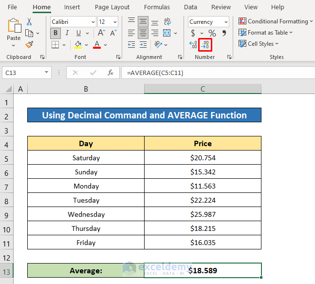
Now see, there are two digits after the decimal and it’s rounded too.

Read More: How to Use Nested IF Function in Excel
Download Practice Workbook
You can download the free Excel workbook from here and practice on your own.
Conclusion
I hope the procedures described above will be good enough to nest a formula with ROUND and AVERAGE functions in Excel. Feel free to ask any question in the comment section and please give me feedback.
<< Go Back to Nested Formula | Excel Formulas | Learn Excel
Get FREE Advanced Excel Exercises with Solutions!
