If you want to create a nested formula in Excel, you have come to the right place. Here, we will walk you through 3 easy examples to do the task smoothly.
What Is a Nested Formula?
When a function stays inside another function and acts as one of the arguments; then it is called a nested formula. Nested formulas are useful to avoid step-by-step calculations, and it is helpful to make calculations in one step rather than making a number of calculations to get to our expected answer.
How to Create a Nested Formula in Excel: 3 Easy Examples
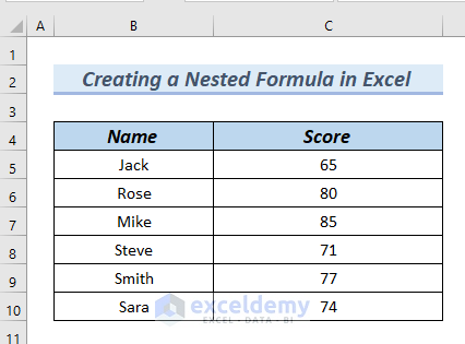
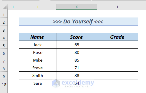
In the following dataset, you can see the Name and Score columns. Using this dataset, we will go through 3 easy examples to create a nested formula in Excel. Here, we used Microsoft Excel 365. You can use any available Excel version.
1. Using IF Function to Create Nested Formula in Excel
In this method, we will use the IF function as an argument inside an IF function to create a nested formula in Excel. After that, using the nested formula, we will find out the Grade of the following dataset.
Steps:
- First, we will type the following formula in cell D5.
=IF(C5>80,"A+",IF(C5>70,"A",IF(C5>60,"C")))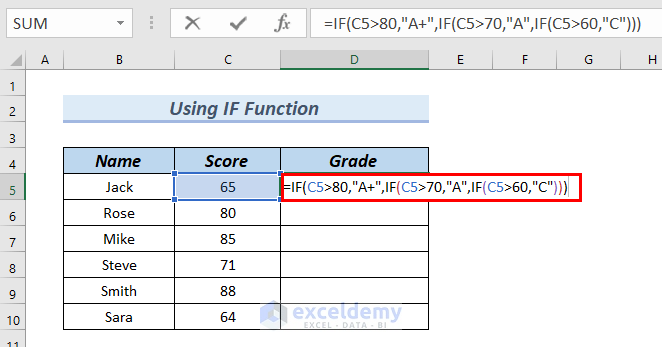
Formula Breakdown
- IF(C5>80,”A+”,IF(C5>70,”A”,IF(C5>60,”C”))) → The IF function makes a logical comparison between a given value and the value we expect. Here, I used nested IF
- IF(C5>60,”C”) → returns “C” when C5>60.
- IF(C5>70,”A”) → returns “A” when C5>70.
- IF(C5>80,”A+”) → returns “A+” when C5>80.
- IF(C5>80,”A+”,IF(C5>70,”A”,IF(C5>60,”C”))) → becomes
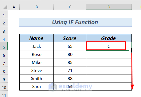
- Output: C
- Explanation: Since the condition C5>60 is true, the IF function returns “C”.
- After that, press ENTER.
Then, you can see the result in cell D5.
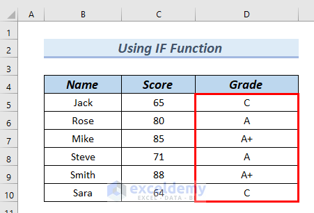
- Furthermore, we will frag down the formula with the Fill Handle Tool.
As a result, you can see the complete Grade column.
Read More: How to Use Nested IF Function in Excel
2. Use of IF, AVERAGE, and MAX Functions
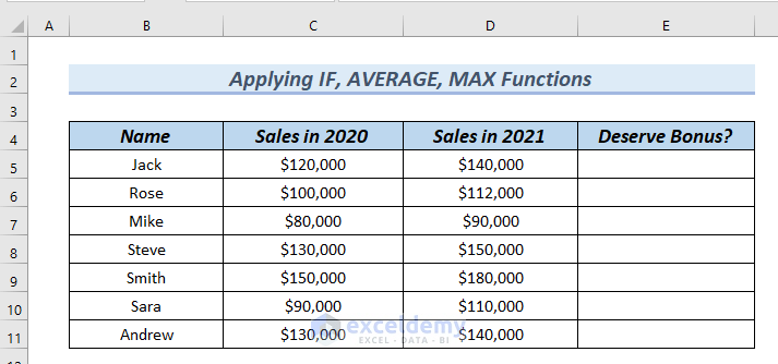
In the following dataset, we can see the Name, Sales in 2020, Sales in 2021, and Deserve Bonus. columns. Next, using the IF, AVERAGE, and MAX functions, we will create a nested formula to find out whether the person in the Name column deserves a bonus or not.
Steps:
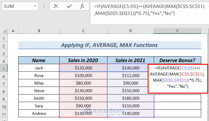
- In the beginning, we will type the following formula in cell E5.
=IF(AVERAGE(C5:D5)>=(AVERAGE(MAX($C$5:$C$11),MAX($D$5:$D$11))*0.75),"Yes","No")
Formula Breakdown
- MAX($C$5:$C$11) → The MAX function returns the maximum value in a range of cells.
- Output: $150,000
- MAX($D$5:$D$11)) → becomes
- Output: $180,000
- AVERAGE(MAX($C$5:$C$11),MAX($D$5:$D$11) → The AVERAGE function returns the average of the values of cells.
- AVERAGE($150,000,$180,000) → becomes
- Output: $165,000
- AVERAGE(MAX($C$5:$C$11),MAX($D$5:$D$11))*0.75 → multiplies $165,000 by 75.
- Output: $123750
- AVERAGE(C5:D5) → becomes
- Output: $130,000
- IF(AVERAGE(C5:D5)>=(AVERAGE(MAX($C$5:$C$11),MAX($D$5:$D$11))*0.75),”Yes”,”No”) → The IF function makes a logical comparison between a given value and the value we expect.
- IF($130,000>= $165,000,”Yes”,”No”) → becomes
- Output: Yes
- Explanation: Since the logical argument of the IF function is true, it returns “Yes”.
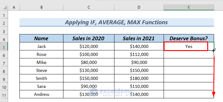
- Afterward, press ENTER.
Therefore, you can see the result in cell E5.
- Moreover, we will frag down the formula with the Fill Handle Tool.
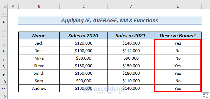
Hence, you can see the complete Deserve Bonus? column.
Read More: How to Use Nested IF and SUM Formula in Excel
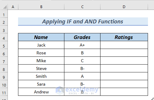
3. Applying IF and AND Functions to Create Nested Formula in Excel
In this method, we will apply the IF and AND functions to create a nested formula in Excel. After that, using the formula we will find out the Ratings in the following dataset.
Steps:
First of all, we will type the following formula in cell D5.
=IF(AND(C5="A+"),"Excellent",IF(AND(C5="A"),"Good","Poor"))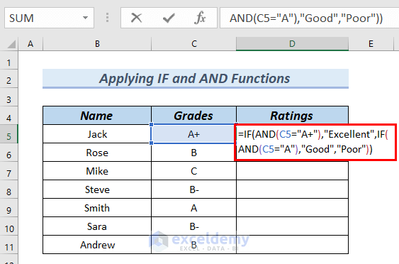
Formula Breakdown
- AND(C5=”A”),”Good”,”Poor”) → The AND function determines whether all conditions in a logical statement are true or not.
- IF(AND(C5=”A+”),”Excellent”,IF(AND(C5=”A”),”Good”,”Poor”)) → the IF function makes a logical comparison between a given value and the value we expect.
- Output: Excellent
- Explanation: Since C5=A+, the formula returns “Excellent”.
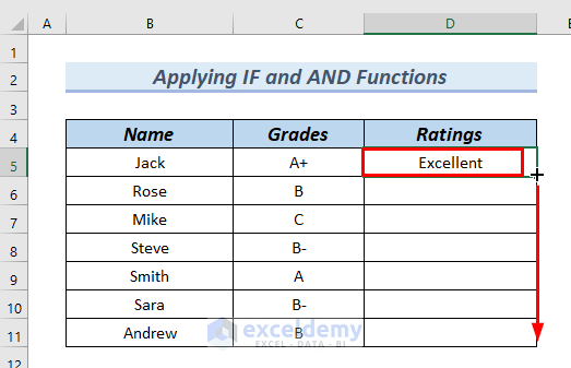
- At this point, press ENTER.
Therefore, you can see the result in cell D5.
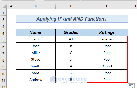
- In addition, we will drag down the formula with the Fill Handle tool.
Hence, you can see the complete Ratings column.
Read More: Nested Formula with AVERAGE and ROUND Functions in Excel
Practice Section
You can download the above Excel file to practice the explained method.
Download Practice Workbook
You can download the Excel file and practice while you are reading this article.
Conclusion
Here, we tried to show you 3 examples to create a nested formula in Excel. Thank you for reading this article, we hope this was helpful. If you have any queries or suggestions, please let us know in the comment section below.
<< Go Back to Nested Formula | Excel Formulas | Learn Excel
Get FREE Advanced Excel Exercises with Solutions!

IF( R5=”1″”F5″,IF(R5=”2″,L5″R5=”3″”M5″)))
HI THERE IM TRYING TO NEST THE ABOVE FORMULA IN A SPREADSHEET BUT STILL CANT GET IT TO WORK.
CAN YOU HELP PLEASE
ROBERT
Hello ROBERT MCPHEE
Thanks for reaching out and posting your query. You wanted to create a nested formula using the IF function. You were almost there. The formula you have given contains some syntax errors.
Corrected Formula:
If you want to use the formula from another sheet, for example, from any sheet and use the R5, F5, L5, and M5 cells of Sheet1, use the following formula.
Hopefully, this idea will help you reach your goal. Good luck!
Regards
Lutfor Rahman Shimanto