How to Use the Multiply Sign (*, the Asterisk) for Multiplication in Excel
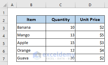
We will use Asterisk (*) to multiply the quantity and unit price for each item in the sample dataset. For that, we have added a new column named Total Price.
- In cell E5, enter the following formula.
=C5*D5It is the alternative to 10*2, we used cell reference instead.
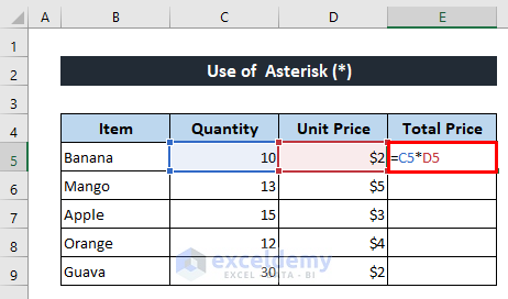
- Press Enter to get the output.
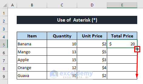
- Drag down the Fill Handle icon to copy the formula for the other items.
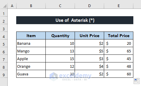
The total price of all the items is calculated by using the multiply sign (*).
Alternatives to Multiply Sign for Multiplication in Excel
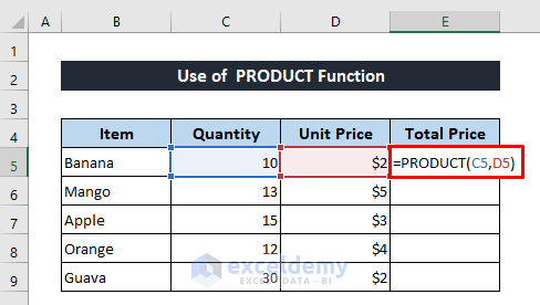
Method 1 – Applying PRODUCT Function to Multiply in Excel
- Enter the following formula in cell E5.
=PRODUCT(C5,D5)It will multiply the value of cells C5 and D5, equivalent to 10*2. If you want to multiply three values of cells C5, D5 and E5, the formula will be:
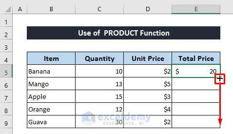
=PRODUCT(C5,D5,E5)- Press Enter to get the result.
You will get the same output as the output of using Asterisk (*).
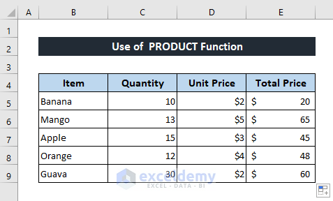
- Use the Fill Handle tool to copy the formula.
- It will output all the results.
Read More: How to Type Math Symbols in Excel
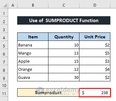
Method 2 – Inserting Excel SUMPRODUCT Function to Multiply
- In cell D11, enter the following formula.
=SUMPRODUCT(C5:C9,D5:D9)- Press Enter.
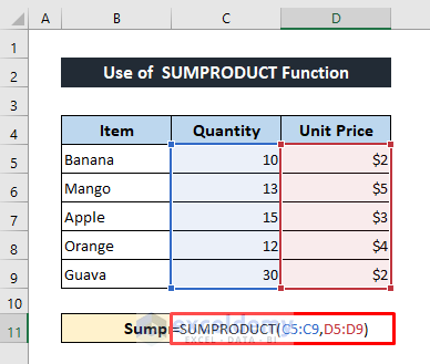
- It will display the output of the sum product.
Read More: How to Add Symbol Before a Number in Excel
3. Using Paste Special Tool to Multiply in Excel
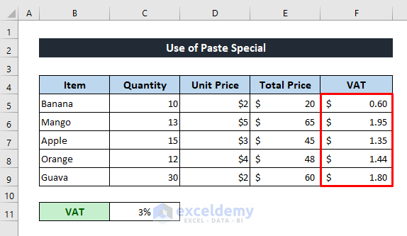
In the sample dataset, we have to pay 3% VAT for each item. To find the amount of VAT for each item, we’ll have to multiply the total values by 3%. Now let’s see how to do it using the Paste Special command.
We have added a new column to the sample dataset to find the VAT.
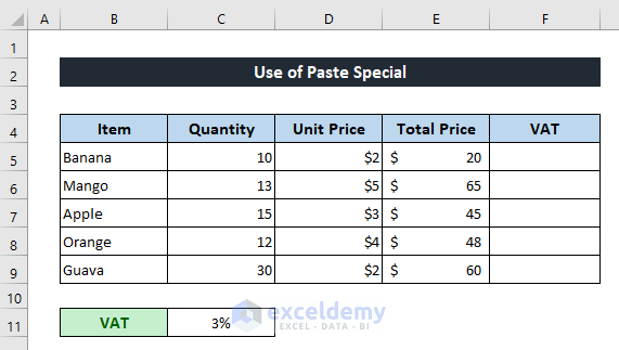
- Copy the Total Prices in the new column using copy and paste.
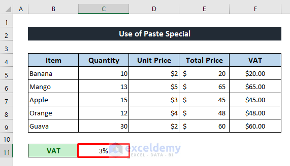
- Copy the VAT value from cell C11.
- Select all the data from the new column and right-click your mouse.
- Press Paste Special from the Context Menu.
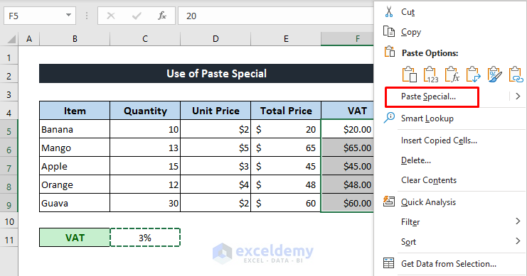
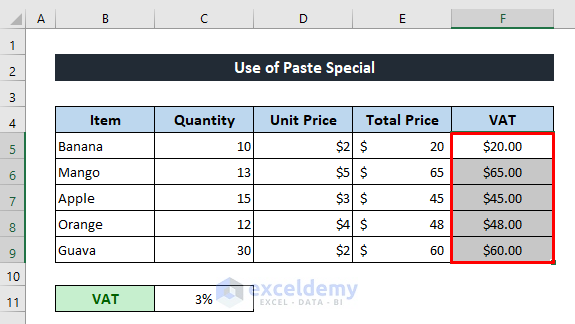
- From the Paste Special dialog box, mark All from the Paste section and Multiply from the Operation section.
- Press OK.

- It will calculate and display the VAT amount for each item.
Read More: How to Put Sign in Excel Without Formula
Download Practice Workbook
Related Articles
- How to Insert Degree Symbol in Excel
- How to Type Diameter Symbol in Excel
- How to Type Math Symbols in Excel
- How to Insert Square Root Symbol in Excel
- How to Insert Less Than or Equal to Symbol in Excel
- How to Insert Greater Than or Equal to Symbol in Excel
- How to Put a Plus Sign in Excel without Formula
- How to Type Minus Sign in Excel Without Formula
- How to Insert Sigma Symbol in Excel
<< Go Back to Mathematical Symbols in Excel | Insert Symbol in Excel | Excel Symbols | Learn Excel
Get FREE Advanced Excel Exercises with Solutions!
