What Is Sankey Diagram?
Sankey diagram is a flow diagram which is handy and effective when working with flow analysis. The width of the arrows is maintained by the quantities and values of the categories.
Any kind of flow analysis such as material flow, energy flow, cash flow, etc. can be visualized and analyzed through this diagram.
Advantages:
- The biggest advantage of the Sankey diagram is you can visualize the trend of multiple categories of your data.
- You can understand the relative weights of every category by the width of the arrows in the Sankey diagram.
- You can portray many complex categories through the Sankey diagram.
Disadvantages:
- It is hard to draw and understand sometimes due to its complex features.
- If the arrow width of the two categories becomes the same, it becomes difficult to differentiate between them.
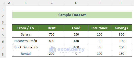
We have a sample dataset of a person’s income source and expenses. We’ll create a Sankey diagram showing how his different income sources cover his expenses.
Step 1 – Preparing Necessary Data to Make Sankey Diagram in Excel
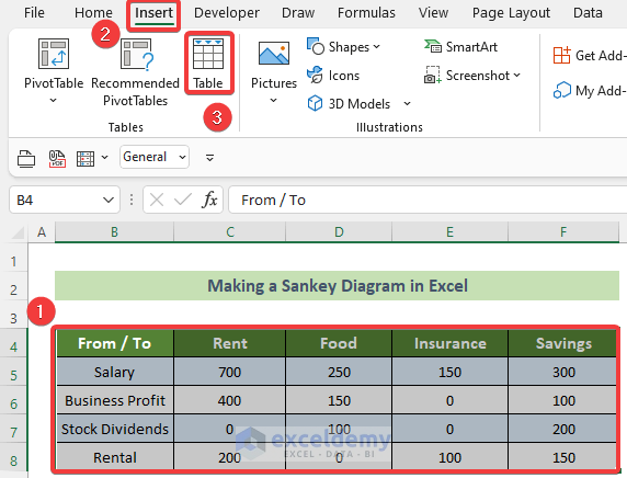
- Select the data range (B4:F8) >> click on the Insert tab >> Table tool.
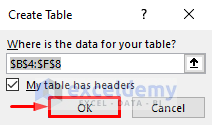
- The Create Table window will appear. Click on the OK button.
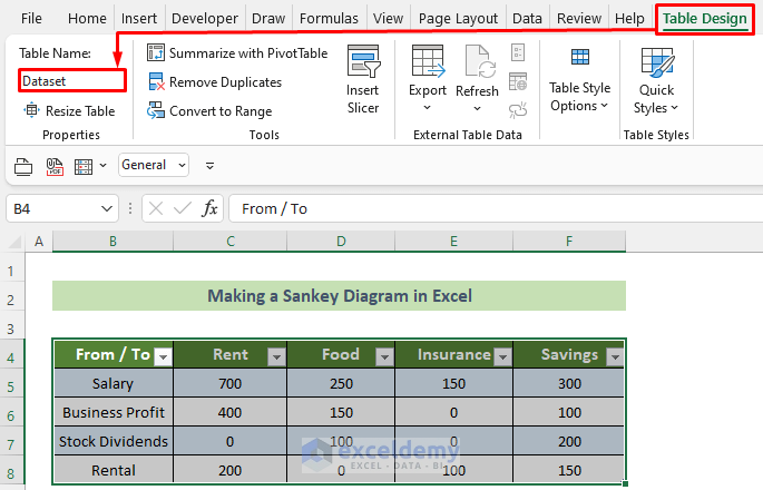
- Name your table.
- Click inside the created table >> go to the Table Design tab >> enter Dataset inside the Table Name:
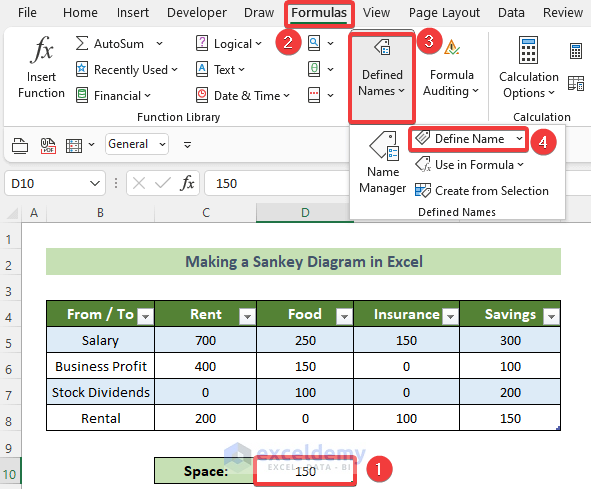
- You need to specify the space between the two categories of the Sankey diagram.
- Enter the value inside the D10 cell >> go to the Formulas tab >> Defined Names group >> Define Name.
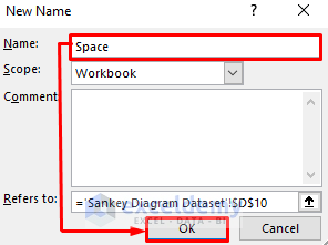
- In the New Name window, enter Space inside the Name: text box and click OK.
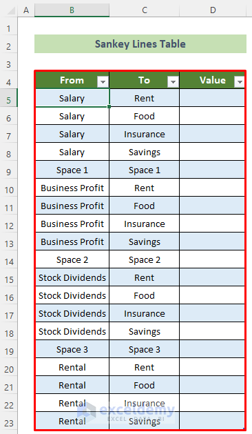
Step 2 – Prepare Sankey Lines Table
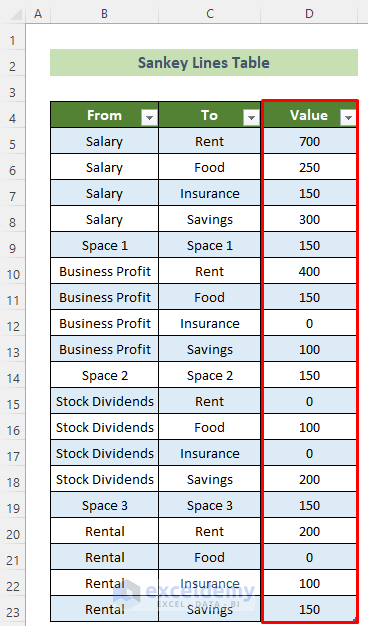
- Create a table named Lines containing From, To and Value columns.
- Click on cell D5 and insert the following formula.
=IF(LEFT([@From],5)="Space",Space,INDEX(Dataset,MATCH([@From],Dataset[From / To],0),MATCH([@To],Dataset[#Headers],0)))- Press Enter.
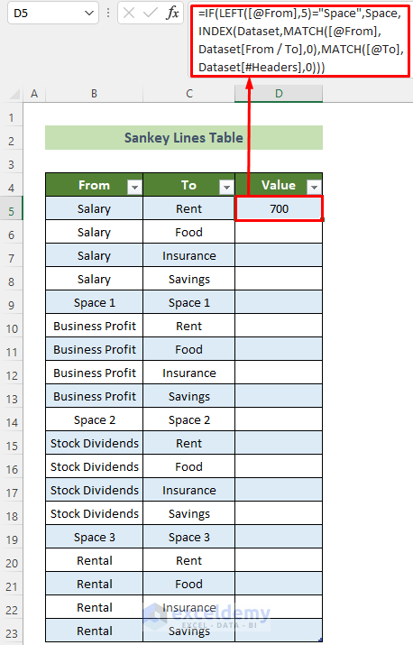
- As this is a table, all the cells below this column will follow the same formula and will be automatically filled.
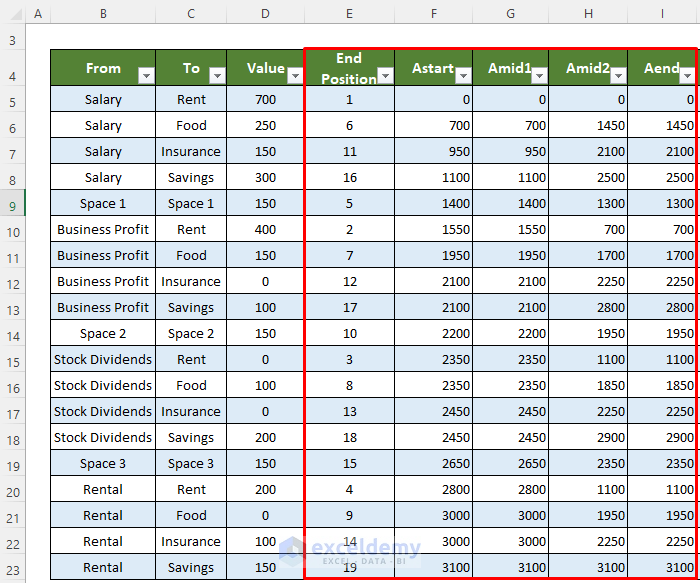
- We have added some new columns and named them End Position, Astart, Amid1, Amid2, Aend, Vstart, Vmid1, Vmid2, Vend, Bstart, Bmid1, Bmid2, and Bend for obtaining values to draw the charts.
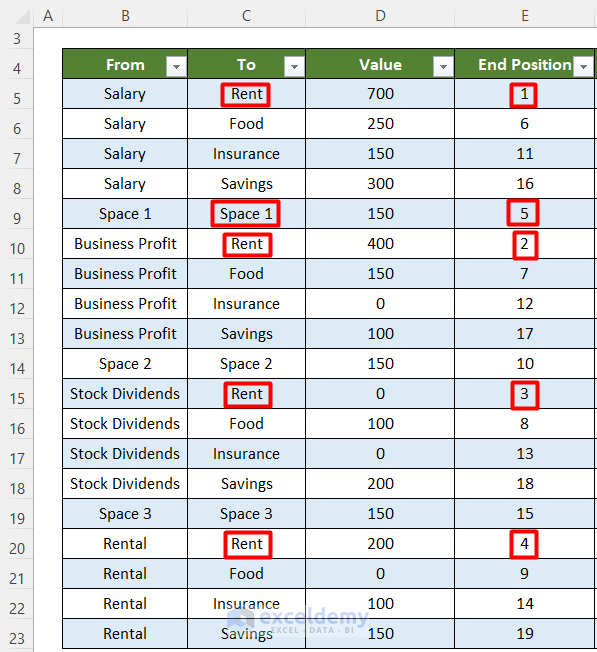
- The values in the End Position column will be given according to column To and insert a space number after each category ends.
- The first category is Rent in the To So, numbering will continue as 1,2,3,4 downwards for Rent and when all Rent is counted, Space 1 will appear and contain the next digit (5 here).
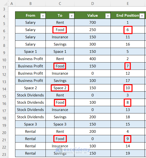
- Food is the second category. It will contain end position numbers from 6. The numbering will increase as we go downward in the To column and find the Food When all the Food category is counted, Space 2 will appear and contain the next digit (10 here). This will go on until all the values of the To column are counted.
- To get the values of the other created columns, enter the following formula and press Enter.
Astart Column:
=SUM(Lines[[#Headers],[Value]]:[@Value])-[@Value]Amid1 Column:
=[@Astart]Amid2 Column:
=[@Aend]Aend Column:
=SUM([Value])-SUMIFS([Value],[End Position],">="&[@[End Position]])Vstart Column:
=[@Value]Vmid1 Column:
=[@Value]Vmid2 Column:
=[@Value]Vend Column:
=[@Value]Bstart Column:
=SUM([Value])-[@Astart]-[@Vstart]Bmid1 Column:
=SUM([Value])-[@Amid1]-[@Vmid1]Bmid2 Column:
=SUM([Value])-[@Amid2]-[@Vmid2]Bend Column:
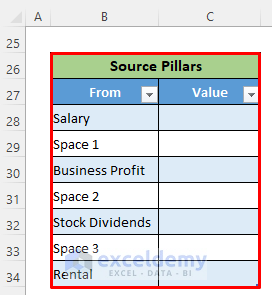
=SUM([Value])-[@Aend]-[@Vend]- Create another table for obtaining the source pillars.
- Create two columns named From and Value in this table.
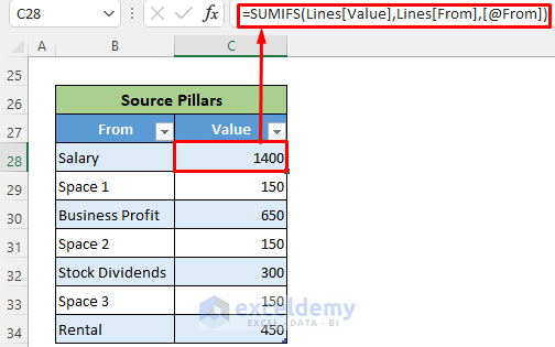
- Click on the C28 cell and enter the following formula for source pillar values.
=SUMIFS(Lines[Value],Lines[From],[@From])- Press Enter.
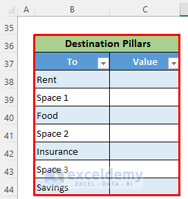
- Create another table for destination pillars with two columns named To and Value.
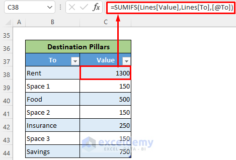
- Click on the C38 cell and enter the following formula.
=SUMIFS(Lines[Value],Lines[To],[@To])- Press the Enter button to get all the destination pillars’ values.
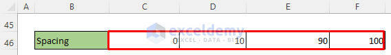
- You will need spacing values of the X-axis to draw the diagram properly.
- Enter the spacing values as 0, 10, 90 and 100 at C46, D46, E46 and F46 cells.
You have all the values that you need to draw the Sankey diagram of your dataset.
Step 3 – Drawing Individual Sankey Lines in Excel
After getting all these values, you need to draw individual Sankey lines.
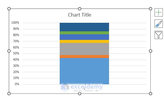
- Click on the Insert tab >> Insert Line or Area Chart tool >> 100% Stacked Area.
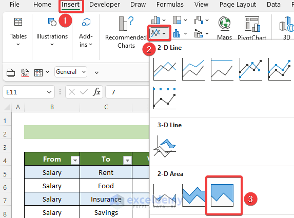
- A 100% stacked area chart will pop up.
- Right-click on the chart area and choose the option Select Data… from the context menu.
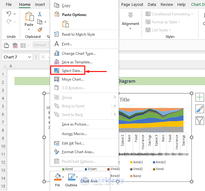
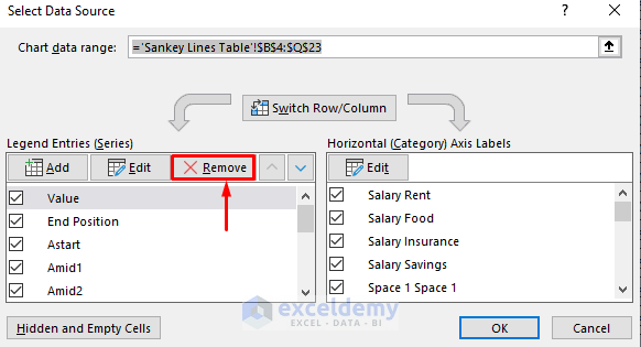
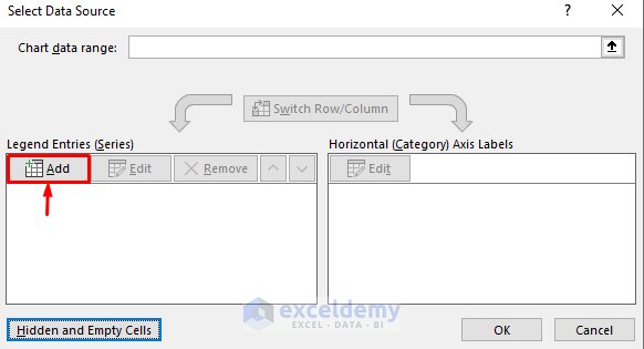
- The Select Data Source window will pop up.
- In the Legend Entries (Series) pane, click on the Remove button to delete all the initial entries.
- Afterward, click on the Add button.
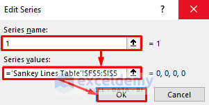
- The Edit Series window will pop up.
- Enter 1 at the Series Name: text box >> choose the F5:I5 cells reference in the Series values: text box.
- Click on OK.
- In the Horizontal (Category) Axis Labels pane, click on Edit.
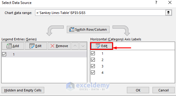
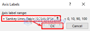
- The Axis Labels window will pop up.
- Refer to the F46:I46 cells in the Axis label range: text box.
- Click on OK.
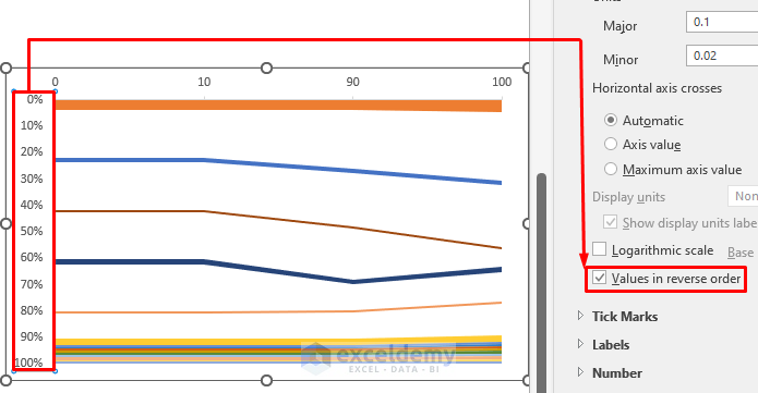
- Double-click on the Y-axis >> tick the option Values in reverse order from the Format Axis pane on the right side.
The Sankey lines are drawn.
Read More: How to Draw Lines in Excel
Step 4 – Adding Sankey Pillars to the Diagram
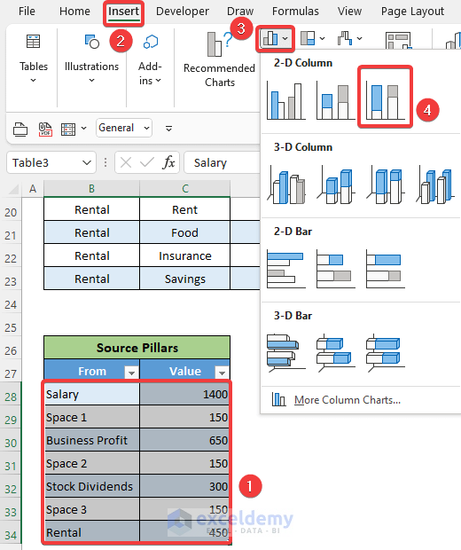
- Select the B28:C34 cells >> click on the Insert tab >> Insert Column or Bar Chart tool >> 100% Stacked Column.
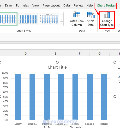
- In the stacked chart window, go to the Chart Design tab >> Change Chart Type.
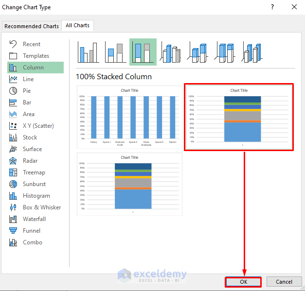
- In the Change Chart Type window, choose the second option and click on OK.
- You will see your desired pillar which will be displayed like the following image.
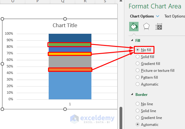
- Since you don’t need the space to be shown, click on the space area and choose the option No fill from the Format Chart Area pane on the right side.
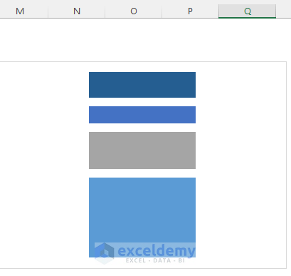
- You will get your final source pillar to make the Sankey diagram.
- You can make pillars for destination sources and change their colors by choosing the Fill Color option from the Format Data Series pane on the right side.

- Combine these Sankey lines with the Sankey pillars to complete the Sankey diagram.
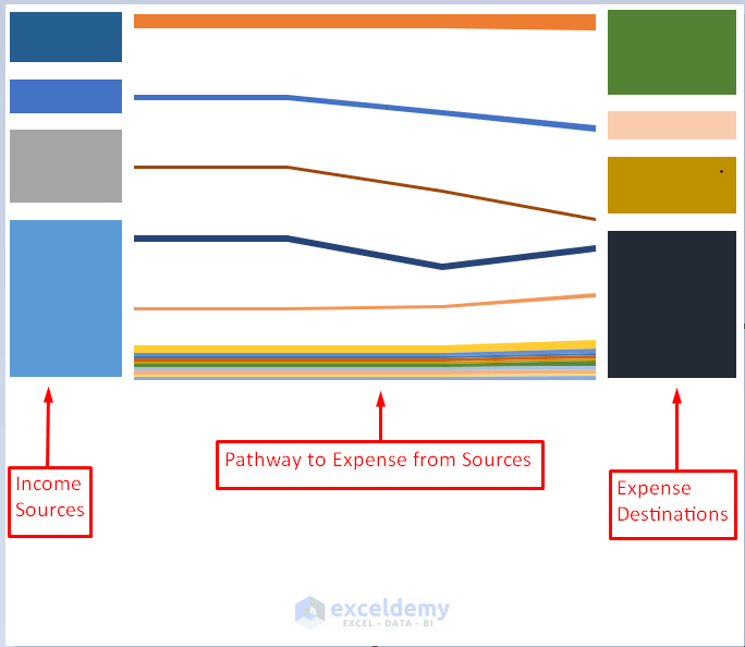
The final diagram will look like the image shown below.
Read More: How to Draw to Scale in Excel
Understanding a Sankey Diagram
Sankey diagrams can easily portray the sources, destinations and contributing pathways from sources to destinations.
Generally, the sources are situated on the left side and the destinations are on the right. From the sources to destinations, several pathways are drawn to depict the tradition and contribution of each source and destination. Besides, the width of these pathways helps to visualize the greater and lesser contribution of pathways.
Read More: How to Make Fishbone Diagram in Excel
Download Practice Workbook
Related Articles
- How to Draw Isometric Drawing in Excel
- How to Draw Shapes in Excel
- How to Remove Unwanted Objects in Excel
- How to Draw Engineering Drawing in Excel
- How to Draw a Floor Plan in Excel
<< Go Back to Drawing in Excel | Learn Excel
Get FREE Advanced Excel Exercises with Solutions!

D5 formula does not work. The syntax of the name “@To” isn’t correct. Verify the name: -starts with a letter or underscore, – Doesn’t include a space or character that isn’t allowed. – Doesn’t conflict with an existing name in the workbook.
Hello James,
Thank you for your query.
Regarding your problem, I can assure you that the formula in cell D5 is correct. The syntax “@To” is not a common syntax, this is right. It is actually a dynamic table formula syntax. When you work with dynamic table formula, then to look up certain column values, you have to use this syntax. Even, if you select a cell of a table column inside a table, you will see the formula would automatically pick this syntax. I hope this answers your question.
Again, to assure you, the formula in cell D5 is working correctly in my file. But, if you keep facing issues regarding this formula, I would really appreciate it if you send me your Excel file. Maybe I can help you further then!
Thank you!
Regards,
Md. Tanjim Reza Tanim
Team Leader, Exceldemy.
I have completed all the other steps but am confused by the ‘end position’ column in the lines table. I do not see a step which tells me what to enter into this column, which is an issue for the other formulas.
I have completed all the other steps but am confused by the ‘end position’ column in the lines table. I do not see a step which tells me what to enter into this column, which is an issue for the other formulas.
Dear FRANCESCA BATHE,
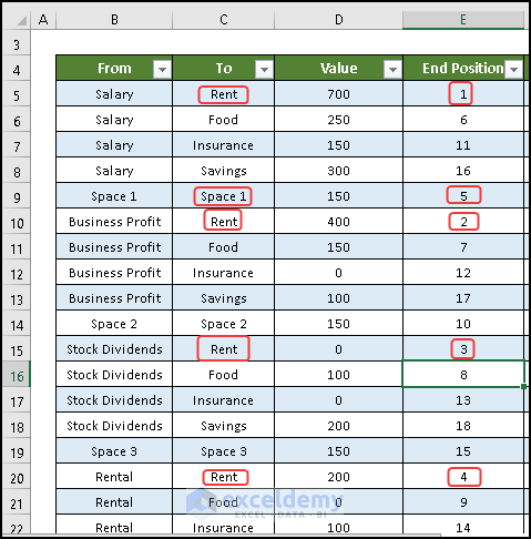
End Position is given according to column To. Where there is RENT in To column, the number starts 1,2,3,4 and ends with SPACE1 numbered 5. Then next is Food starting 6,7,8, 9 and ends with SPACE2 numbered 10. Likewise, numbering is done for every cell data in End Position.
Regards,
Joyanta Mitra