How to Make Fishbone Diagram in Excel: 6 Easy Methods

You can use the Shape feature to make the Fishbone diagram in Excel.

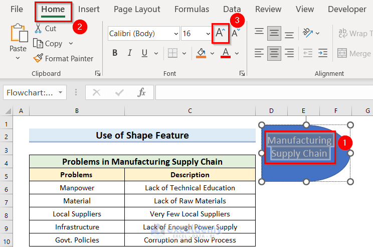
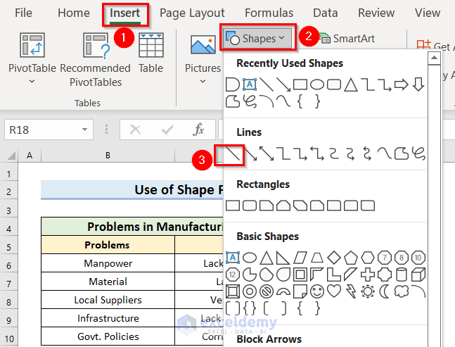
Step 1 – Inserting the Fish Head

• From the Insert tab, go to the Shapes feature.
• Select the Delay shape which is in the Flowchart section.

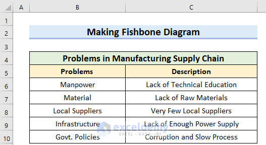
• Drag the Mouse Pointer where you want to keep the Fish Head. 

• Double-click on the shape and you will see the Text Bar.

• Write the focus words of the diagram. We have written “Manufacturing Supply Chain”.

• You can change the Shape’s location by dragging the Mouse Pointer.

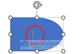
Step 2 – Formatting Text in the Fish Head

• Select the Text.
• From the Home tab, go to the Alignment feature. We have done Center and Middle alignment.

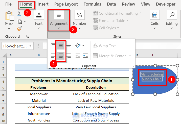
• Change the Font Size. We have increased the Font Size to 16.

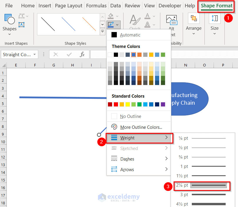
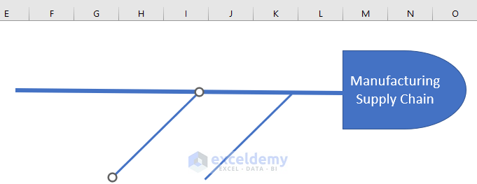
Step 3 – Including the Main Bone

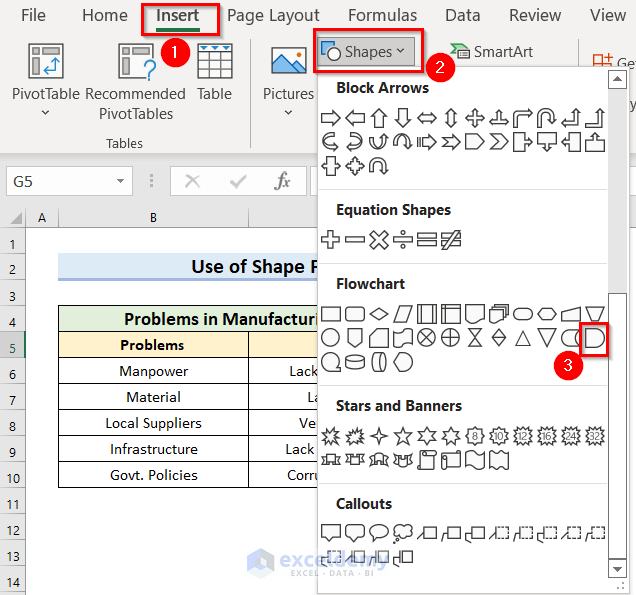
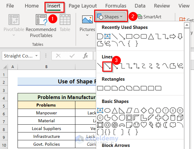
• From the Insert tab, go to the Shapes feature.
• From the Lines command, select the Line shape.

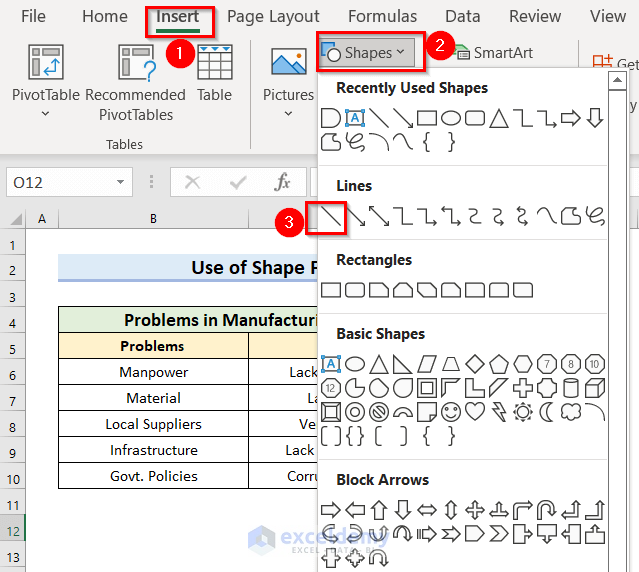
• Drag the Mouse Pointer towards the Fish Head. 
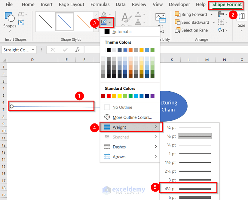
• From the Shape Format tab, go to the Shape Outline.
• From the Weight option, choose your preferred line weight. Choose a weight that will keep the diagram visible.

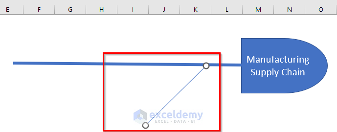
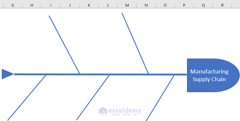
You will get the following output.

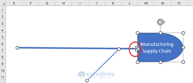
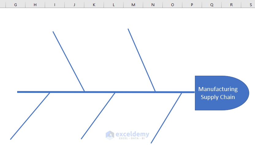
Step 4 – Adding Fish Bones

• From the Insert tab, go to the Shapes feature.
• From the Lines command, select the Line shape.

• Drag the Mouse Pointer towards the Fish Head and Main Bone. 

• Select the shape.
• From the Shape Format tab, go to the Shape Outline.
• From the Weight option, choose your preferred line weight. Choose a weight that will keep the diagram visible. Keep this thinner than the Main Bone.

Move the whole diagram by selecting all those shapes using the Ctrl key.

• Draw more bones or copy the bone using Excel keyboard shortcuts Ctrl + C and then paste the bone by pressing the Ctrl + V keys. This is the easiest way to add lots of bones.

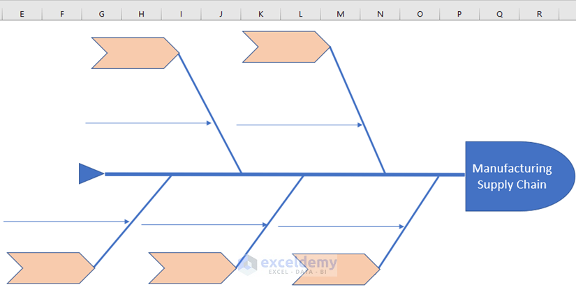
You will see the following shapes.

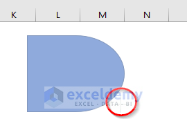
Step 5 – Inserting the Fish Tail to Make the Fishbone Diagram in Excel

• From the Insert tab, go to the Shapes feature.
• Select the Isosceles Triangle shape, which is in the Basic Shapes section.

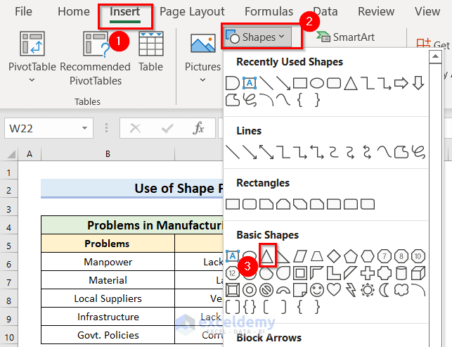
• Drag the Mouse Pointer where you want to keep the Fish Tail. 
• Rotate the shape to look like a Fish Tail.

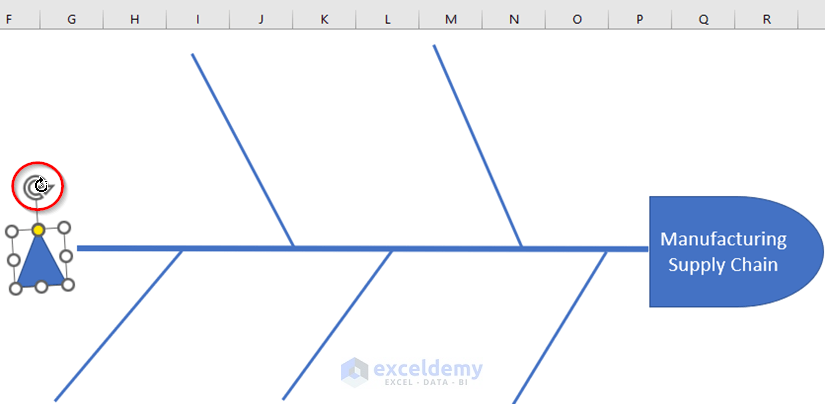
You will get the Fishbone Shape.

Step 6 – Including the Chevron Arrow to Narrate Data for Making the Fishbone Diagram

• From the Insert tab, go to the Shapes feature.
• From the Block Arrows option, select the Chevron arrow shape.

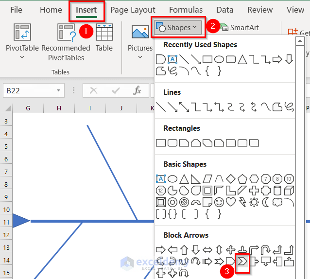
• Drag the Mouse Pointer where you want to keep the shape.
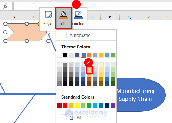
• Right-click on the shape.
• From the Context Menu Bar, go to Fill and change the fill color. We have chosen Orange, Accent 2, Lighter 60%.

• Draw more Chevron arrows or use Ctrl + C to copy them and Ctrl + V to paste them.

Step 7 – Placing Line Arrows

• From the Insert tab, go to the Shapes feature.
• From the Lines command, select the Line Arrow shape.

• Drag the Mouse Pointer towards the Fish Bones. 

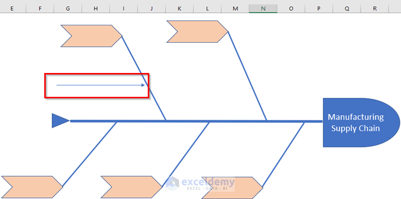
• Draw more Line Arrows or copy-paste them.

Steo 8 – Inserting Data in Fishbone Diagram

• Write the data inside the Chevron arrows.

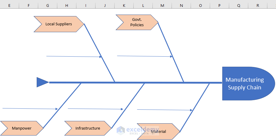
Describe the causes you should use the Text Box feature.

• From the Insert tab, go to the Text command.
• Click the Text Box feature.

• Drag the Mouse Pointer above the Line Arrow. 

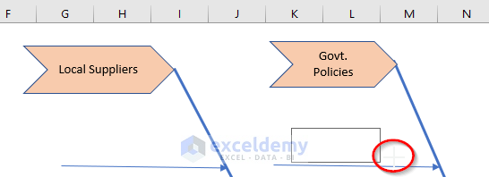
• Write the description in the box.
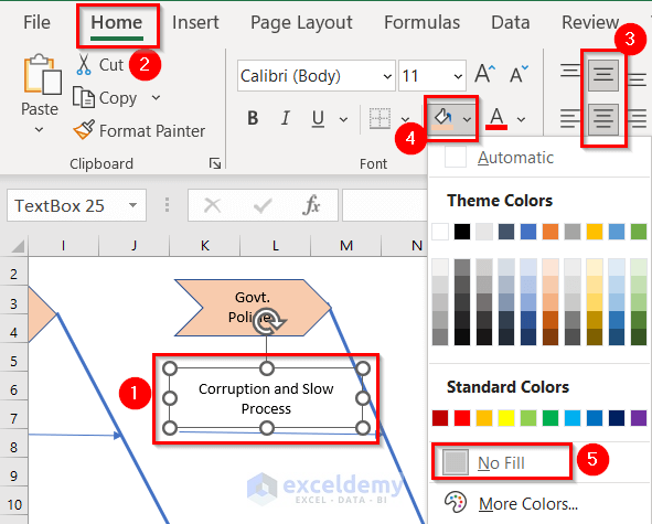
• Select the box.
• From the Home tab, change the Alignment to Middle and Center.
• From the Fill option, choose No Fill.

• Write the description for the other arrows.

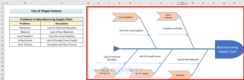
We have attached a clear view of the Ishikawa diagram.

Download the Practice Workbook

Related Articles

• How to Draw Isometric Drawing in Excel
  
• How to Draw Shapes in Excel
• How to Remove Unwanted Objects in Excel
• How to Draw Engineering Drawing in Excel
• How to Draw a Floor Plan in Excel

<< Go Back to Drawing in Excel | Learn Excel