How to Insert a Stacked Column Pivot Chart in Excel

If we insert a Stacked Column chart from Pivot Table then it has some advantages instead of using a general Stacked Column. Such as Pivot Table provides the total sum for each section automatically and we’ll get it in our stacked column chart too. The inserting procedures are quite easy. You will learn the procedures to insert a Stacked Column Pivot Chart in Excel from this article with proper images for every step.

Download Practice Workbook

You can download the free Excel workbook from here and practice independently.

What Is Stacked Column Pivot Chart?

When we insert the Stacked Column chart from the Pivot Table instead of inserting it from the normal range then it is called a Stacked Column Pivot Chart.

Easy Steps to Insert a Stacked Column Pivot Chart in Excel

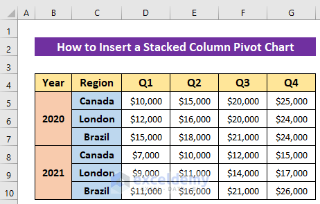
Now we’ll learn the easy steps to make a Stacked Column Pivot Chart. Before starting get introduced to our dataset which represents the quarterly sales for three regions of a company.

First, we’ll convert a normal range to a Pivot Table then we’ll insert a Stacked Column Pivot Chart.

Steps:

• Select any cell from the data range.
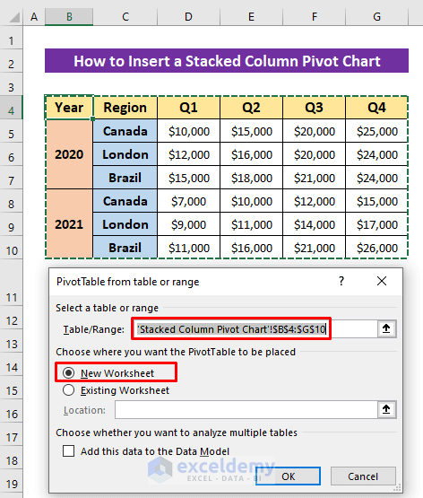
• Then click as follows: Insert > Pivot Table.

Soon after, a dialog box will open up and it will automatically select the whole data range.

• Mark required worksheet option. I marked New Worksheet.
• Next, just press OK.

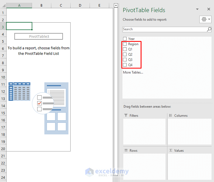
After a while, a new worksheet will open up with PivotTable Fields.

• Mark the quarters and Region options.

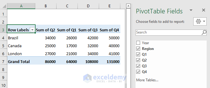
Soon you will see that a Pivot Table has been created as in the image below.

We have reached our final step- inserting a Stacked Column chart.

• Click according to the serial: Insert > Insert Column or Bar Chart > Stacked Column.

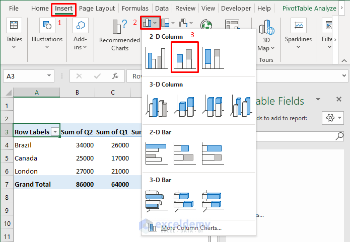
Here’s our Stacked Column Pivot Chart. It is showing the sum of every quarter with different colors as a column. So from this graphical representation, we can easily understand the difference between the sum of quarters just by looking at a glance.

Read More: Difference Between Pivot Table and Pivot Chart in Excel

Customize Stacked Column Pivot Chart in Excel

Excel offers huge customization for your charts so that you can modify them according to your requirements. So now, we’ll learn some major and most useful customizations.

Hide All Field Buttons from Chart

Maybe you have already seen that the Pivot fields are also available in the Stacked Column Pivot Chart. This feature is not available in the general Excel Charts. So it’s one of the important advantages of the Stacked Column Pivot Chart. But if you think that it’s not necessary for you then you can easily hide it.

Steps:

• First, right-click on any field name on the Pivot Chart.
• After that, select the Hide All Field Buttons on Chart option from the appeared context menu.

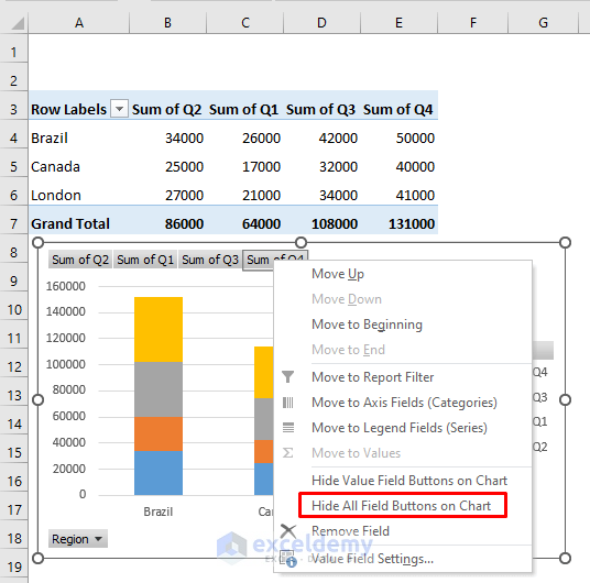
Now see, all the fields are gone and the chart is looking clean.

Read More: How to Use Pivot Chart in Excel (8 Suitable Examples)

Change Column Gap Width

If you want to change the gap between the columns then it is also possible in a Stacked Column Pivot Chart.  If we decrease the gap it may look better.

Steps:

• Double click on any cluster of the stacked columns and a field named Format Data Series will appear on the right side of the Excel sheet.
• Then set the gap from the Gap Width option. I set 20%.

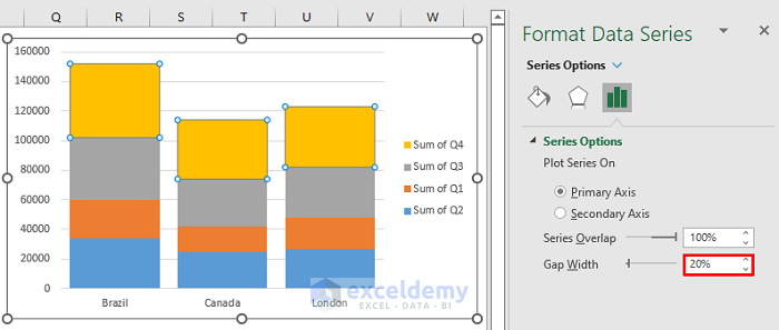
See, the gap has decreased and the width of the columns increased.

Edit Cluster Border

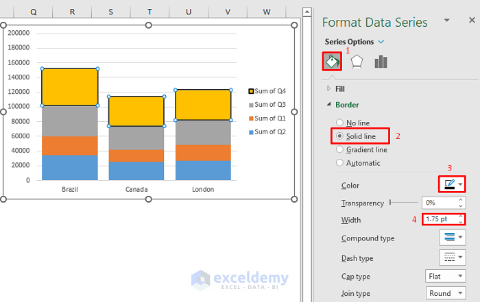
For every cluster of the Stacked Column, you can create a border. Borders give a better look at the chart or you can highlight specific clusters by giving a border.

Steps:

• Double click on the cluster to that you want to add a border.
• Then click on the Fill & Line option.
• Next, mark Solid Line, choose the desired color, and set the width. I chose black color and width- 1.75pt.

• Do the same operation for the other clusters of the Stacked Columns.

Then your chart will look like the image below.

Format Vertical Axis

We can set the minimum and maximum bounds for the chart by formatting the vertical axis.

Steps:

• Double click on the vertical axis to open the Format Axis field.
• Later, set the minimum and maximum range. I kept the minimum bound at zero and set the maximum bound at 200000.

It’s the output image after setting the new bound.

Change Chart Design

Excel has some built-in chart designs. From there, you can choose your best-suited chart.

Steps:

• Select the chart by clicking anywhere on the chart.
• After that click on the Design ribbon and select your required chart design. I chose- Style 2.

Now have a look at this chart design showing the data of the vertical axis in it.

Read More: How to Import Data into PowerPivot & Create Pivot Table/Pivot Chart

Change Color

In any chart design, you can change the colors of the cluster in the columns. So if you don’t like the default color of your chart then you can easily change them.

Steps:

• Firstly, click as follows: Design > Change Colors and then select your desired color collections from the drop-down menu. I picked Colorful Palette 3.

Now you see, the new colors applied successfully and it’s looking pretty cool, right?

Conclusion

That’s all for the article. I hope the procedures described above will be good enough to insert a stacked column pivot chart in Excel. Feel free to ask any questions in the comment section and give me feedback. Visit ExcelDemy to explore more.

Related Articles

• How to Edit Pivot Chart in Excel (with Easy Steps)
• How to Refresh Pivot Chart in Excel (4 Suitable Approaches)
• How to Add Target Line to Pivot Chart in Excel (2 Effective Methods)
• How to Filter a Pivot Chart in Excel (5 Suitable Ways)
• How to Make a Bar Graph in Excel with 2 Variables (3 Easy Ways)
• How to Filter a Pivot Chart in Excel (5 Suitable Ways)
• How to Make a Bar Graph in Excel with 2 Variables (3 Easy Ways)