How to Filter a Pivot Chart in Excel (5 Ways)

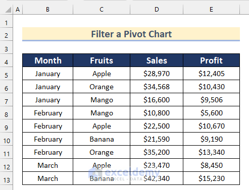
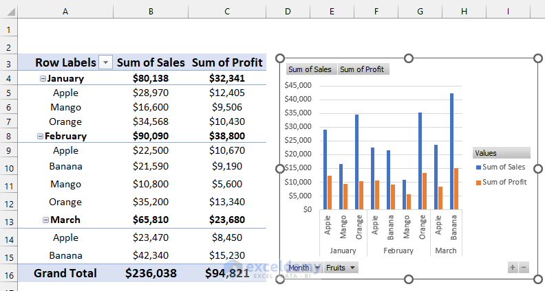
We have a dataset containing a shop’s Month, Fruits, Sales, and Profit. We will use this dataset to show you how to filter a pivot chart in Excel.

Method 1 – Using Field Buttons to Filter a Pivot Chart in Excel

Steps:

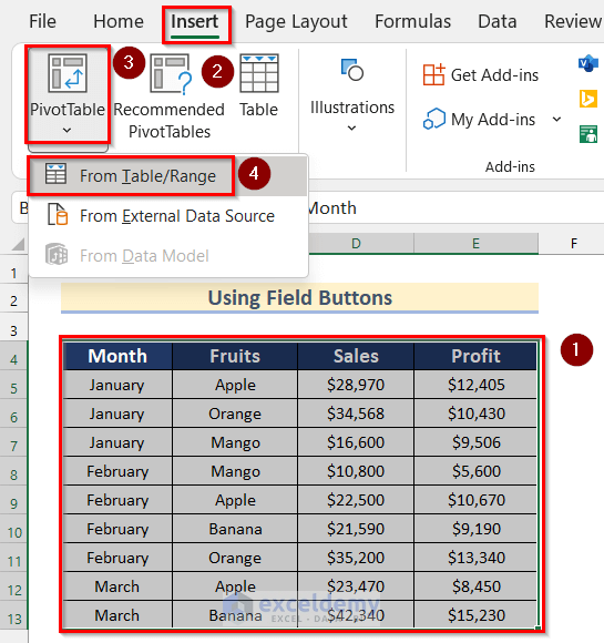
• Select the cell range B4:E13.
• Go to the Insert tab >> click on PivotTable >> select From Table/Range.

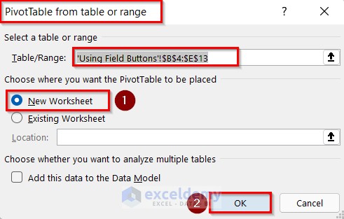
• The PivotTable from table or range box will open.
• You can see that the cell range B4:E13 has already been selected in the Table/Range box.
• Select New Worksheet.
• Press OK.

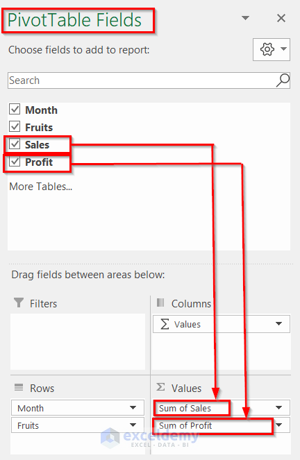
• The PivotTable Fields toolbox will appear.
• Insert the Month and Fruits fields into the Rows box.

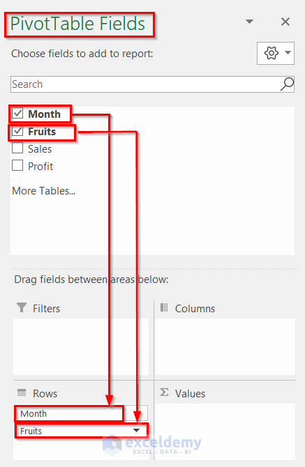
• Insert the Sales and Profit fields into the Values box.

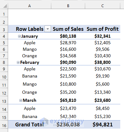
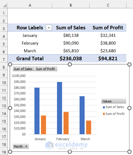
• You can create a pivot table from your dataset.

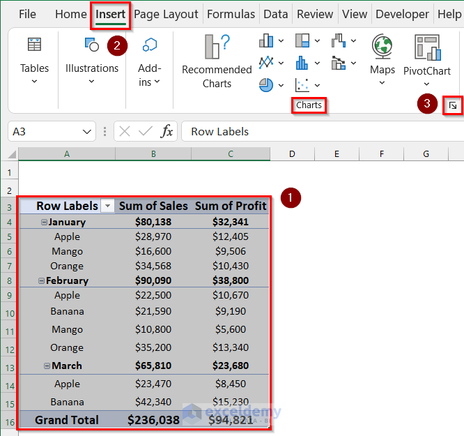
• Select the cell range A3:C16.
• Go to the Insert tab >> From Charts >> click on the Recommended Charts box.

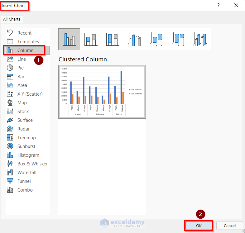
• The Insert Chart box will appear.
• Select any chart of your preference. Here, we selected the Clustered Column chart.
• Press OK.

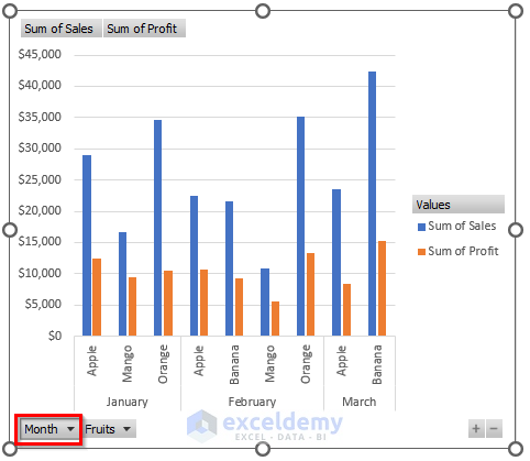
• You can add a Pivot Chart in Excel.

• In the Pivot Chart, you can see the Field Buttons.
• Click on the Month Field Button.

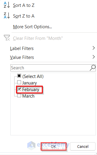
• A Filter box will open.
• Select February only.
• Press OK.

• You will have a filtered Pivot Chart using Field Buttons.

Read More: How to Add Grand Total to Stacked Column Pivot Chart

Method 2 – Dragging Fields in Filter Box

Steps:

• Create a Pivot Chart from a Pivot Table by going through the steps given in Method 1.
• Click on the Pivot Chart.

• Click on the PivotChart Fields box.
• Drag only the Month Field in the Axis box.

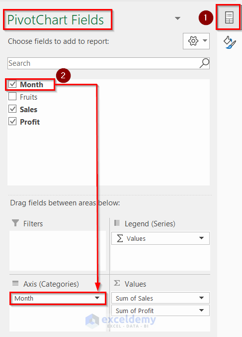
• You will find a Pivot Chart only with the Month Field as Axis.
• You can filter your Pivot Chart by dragging Fields in the Filter Box.

Read More: Create a Clustered Column Pivot Chart in Excel

Method 3 – Using Pivot Tables to FiIter a Pivot Chart in Excel

Steps:

• Create a Pivot Table and Pivot Chart using your dataset by going through the steps given in Method 1.

• Click on the manual filters button in the Row Labels column.

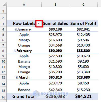
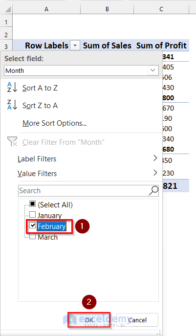
• A Filter box will open.
• Select February only.
• Press OK.

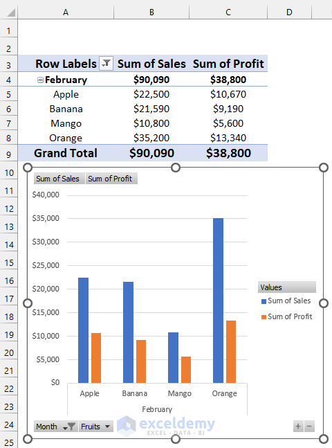
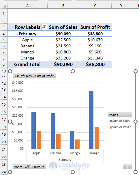
• You will have a filtered Pivot Chart using Pivot Table.

Method 4 – Using a Slicer to Filter a Pivot Chart in Excel

Steps:

• Create a Pivot Table and Pivot Chart using your dataset by going through the steps given in Method 1.

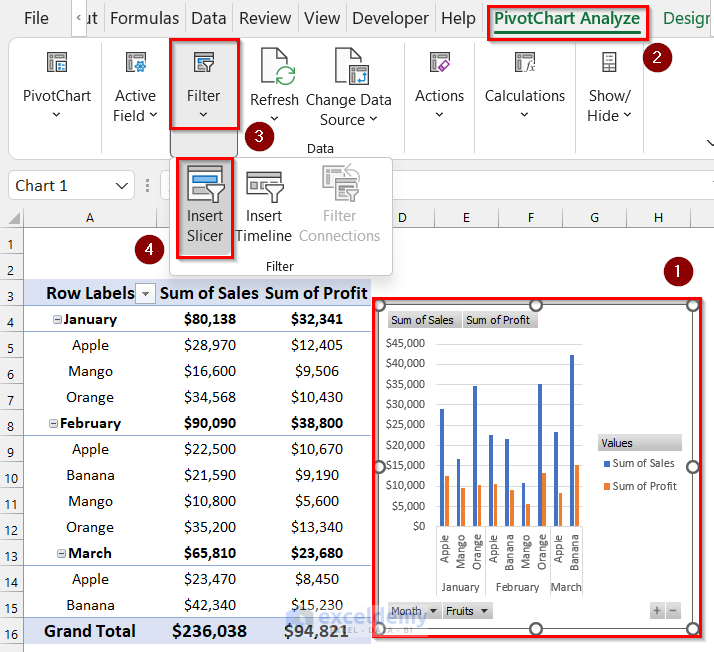
• Select the Pivot Chart.
• Go to the PivotChart Analyze tab >> click on Filter >> select Insert Slicer.

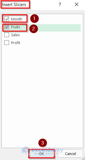
• The Insert Slicer box will appear.
• Select the Month and Fruits fields.
• Press OK.

• You can see that two Slicer boxes for Month and Fruits have opened.

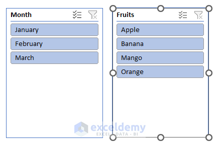
• Select February in the Month box and Banana in the Fruits box.

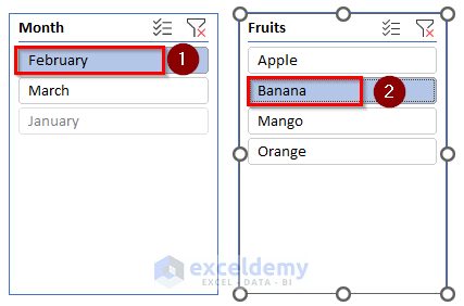
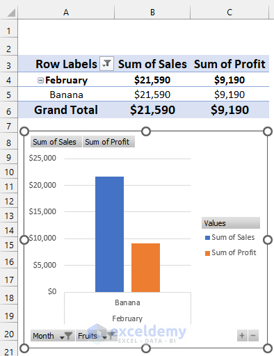
• You will find a Pivot Chart only with the data for February from the Month field and Banana from the Fruits field.
• You can filter your Pivot Chart by dragging Fields in the Filter Box.

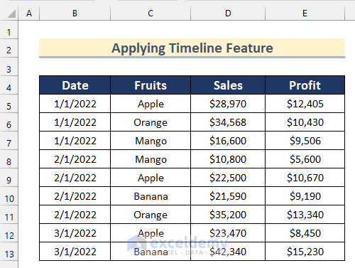
Method 5 – Applying Timeline Feature to Filter a Pivot Chart 

We have a dataset containing some Fruits’ Dates, Sales, and Profits. We will use this data to filter a Pivot Chart by applying the Timeline feature.

Steps:

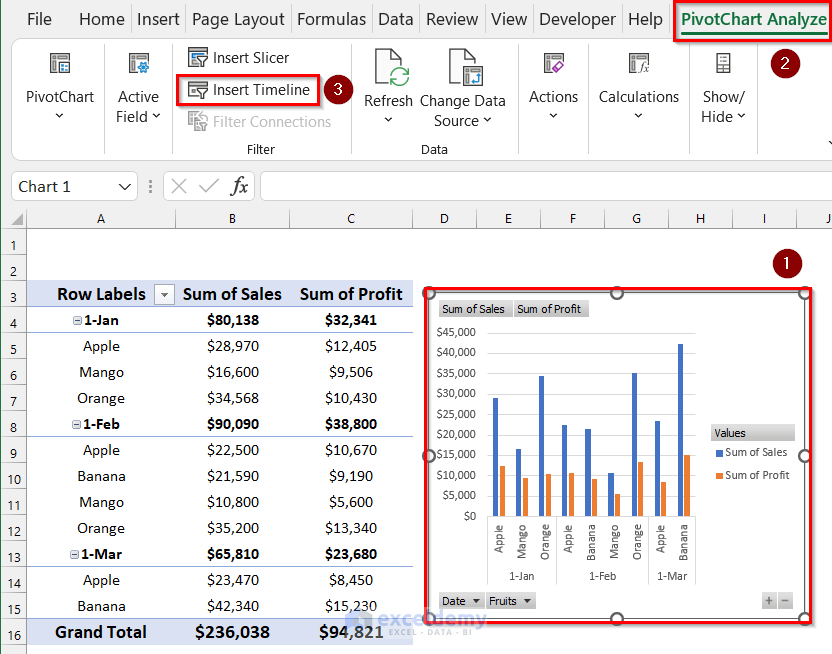
• Create a Pivot Table and Pivot Chart using your dataset by going through the steps given in Method 1.

• Select the Pivot Chart.
• Go to the PivotChart Analyze tab >> click on Insert Timeline.

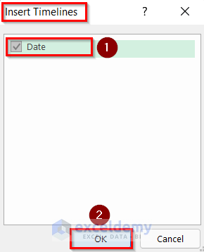
• The Insert Timelines box will appear.
• Click on Date.
• Press OK.

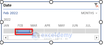
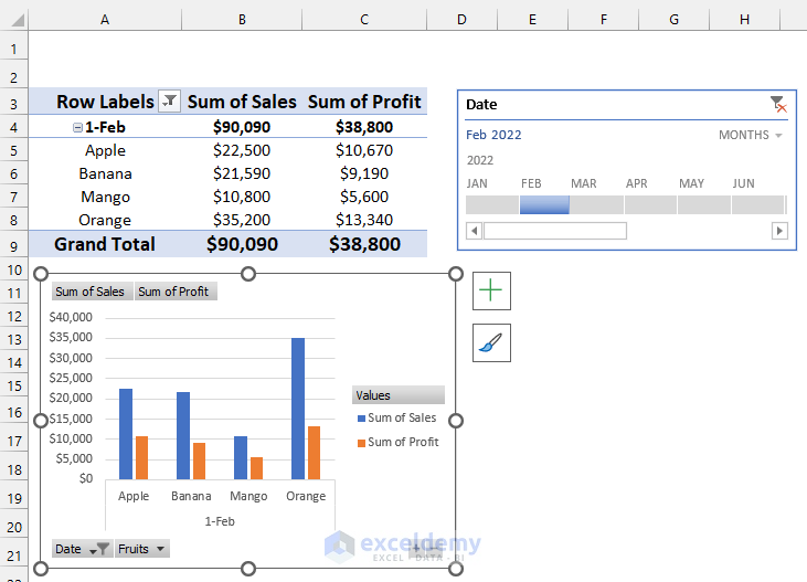
• Click on FEB in the Date box.

• You will have a filtered Pivot Chart with only the value of February by applying the Timeline Feature.

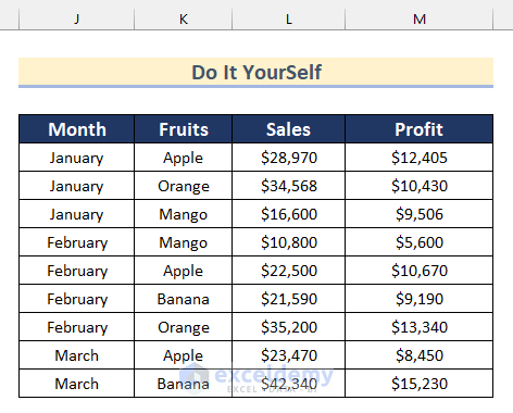
Practice Section

Here is a dataset to practice these methods on your own.

Download the Practice Workbook

Related Articles

• How to Add Target Line to Pivot Chart in Excel
• How to Add Secondary Axis in Excel Pivot Chart
• How to Show Grand Total with Secondary Axis in Pivot Chart

<< Go Back to Pivot Chart | Pivot Table in Excel | Learn Excel