Here’s an overview of using VBA to create a chart from a pivot table.
Use Excel VBA to Create Chart from Pivot Table: 3 Methods
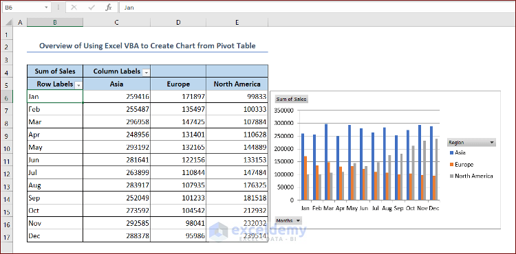
We have the sales data of a company for a specific region on a particular day. The dataset includes the Date, Region and Sales data of different products.

We have created a Pivot Table from the dataset. We have selected the Region, Sales and Months fields for display. In the Columns area, we have put the Region field. In the Rows area, we have put the Months field. The Values area includes the Sum of Sales.

Note: You can follow this article How to Create a Pivot Table in Excel to learn how to create a Pivot Table in Excel.
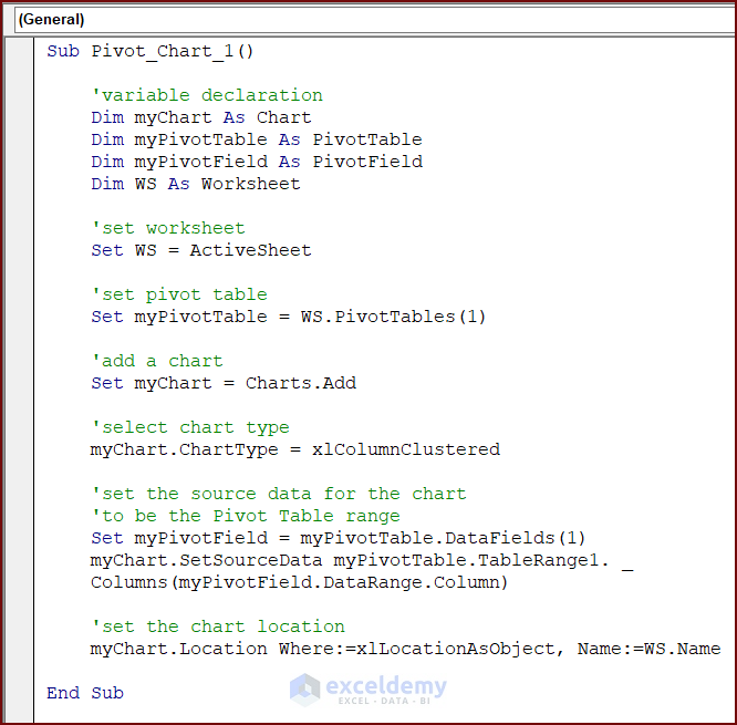
Method 1 – Using the Charts.Add Method
We can use the following VBA code based on Excel VBA Charts.Add method to create a chart from Pivot Table.
- Launch the VBA macro editor from your workbook. Follow this article How to Write VBA Code in Excel.
- Paste the following code in your VBA Editor Module and press the Run button or F5 key to run the code:
Sub Pivot_Chart_1()
    'variable declaration
    Dim myChart As Chart
    Dim myPivotTable As PivotTable
    Dim myPivotField As PivotField
    Dim WS As Worksheet
    'set worksheet
    Set WS = ActiveSheet
    'set pivot table
    Set myPivotTable = WS.PivotTables(1)
    'add a chart
    Set myChart = Charts.Add
    'select chart type
    myChart.ChartType = xlColumnClustered
    'set the source data for the chart to be the Pivot Table range
    Set myPivotField = myPivotTable.DataFields(1)
    myChart.SetSourceData myPivotTable.TableRange1.Columns(myPivotField.DataRange.Column)
    'set the chart location
    myChart.Location Where:=xlLocationAsObject, Name:=WS.Name
End Sub
VBA Breakdown
Sub Pivot_Chart_1()- This line defines the start of a subroutine called Pivot_Chart_1.
    Dim myChart As Chart
    Dim myPivotTable As PivotTable
    Dim myPivotField As PivotField
Dim WS As Worksheet- This section declares several variables used within the subroutine. myChart is declared as Chart, myPivotTable is declared as PivotTable, myPivotField is declared as PivotField, WS is declared as Worksheet object.
Set WS = ActiveSheet- This line of code assigns the currently active worksheet to the WS variable.
Set myPivotTable = WS.PivotTables(1)- This line assigns PivotTables(1) in the WS worksheet to the myPivotTable variable.
Set myChart = Charts.Add- This line adds a new chart and assigns it to the myChart variable.
myChart.ChartType = xlColumnClustered- This line of code sets the chart type of myChart to a clustered column chart. You can choose any chart of your wish.
Set myPivotField = myPivotTable.DataFields(1)- This line assigns the first data field (column) of the myPivotTable to the myPivotField variable.
myChart.SetSourceData myPivotTable.TableRange1.Columns(myPivotField.DataRange.Column)- This section of code sets the source data for the chart to be the column range of the data field in the myPivotTable.
myChart.Location Where:=xlLocationAsObject, Name:=WS.Name- This line sets the location of the chart to be within the worksheet specified by WS.
End Sub- This line marks the end of the subroutine.
Overall, this code creates a new chart, sets its type to a clustered column chart, and links it to a PivotTable in the active worksheet. Then sets the source data for the chart to the column range of the first data field in the PivotTable and specifies the location of the chart within the worksheet.

Note: This chart shows the total sales values for all the regions (Asia, Europe and North America) for all the months. If you wish you can filter the regions from the Regions drop-down. Similarly, you can filter the months from the Months drop-down.
Read More: How to Create Chart from Pivot Table in Excel
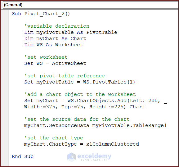
Method 2 – Apply the ChartObjects.Add Method
We can use the following VBA code containing Excel VBA ChartObjects.Add method to create a chart from Pivot Table.
- Paste the following code in your VBA Module and press the Run button or F5 key to run the code:
Sub Pivot_Chart_2()
    ‘variable declaration
    Dim myPivotTable As PivotTable
    Dim myChart As Chart
    Dim WS As Worksheet
    'set worksheet
    Set WS = ActiveSheet
    'set pivot table reference
    Set myPivotTable = WS.PivotTables(1)
    'add a chart object to the worksheet
    Set myChart = WS.ChartObjects.Add(Left:=200, Width:=375, Top:=75, Height:=225).Chart
    'set the source data for the chart to be the Pivot Table range
    myChart.SetSourceData myPivotTable.TableRange1
    'set the chart type
    myChart.ChartType = xlColumnClustered
End Sub
VBA Breakdown
Sub Pivot_Chart_2()- This line defines a new subroutine called Pivot_Chart_2.
    Dim myPivotTable As PivotTable
    Dim myChart As Chart
Dim WS As Worksheet- This code section declares three variables: myPivotTable of type PivotTable, myChart of type Chart, and WS of type Worksheet. These variables will be used to store references to the pivot table, chart, and worksheet objects, respectively.
Set WS = ActiveSheet- This line assigns the active worksheet to the variable WS. The ActiveSheet property returns the currently active worksheet.
Set myPivotTable = WS.PivotTables(1)- This assigns the first pivot table in the worksheet to the variable myPivotTable. The PivotTables property of the worksheet returns a collection of all the pivot tables in that worksheet.
Set myChart = WS.ChartObjects.Add(Left:=200, Width:=375, Top:=75, Height:=225).Chart- This section of code adds a new chart object to the worksheet using the ChartObjects.Add method. The Left, Width, Top, and Height parameters specify the position and size of the chart object. The .Chart property returns the chart embedded within the ChartObject, and that is assigned to the variable myChart.
myChart.SetSourceData myPivotTable.TableRange1- This sets the source data for the chart to be the range of the pivot table using the SetSourceData method. The TableRange1 property of the pivot table returns the entire range of the pivot table data.
myChart.ChartType = xlColumnClustered- This code section sets the chart type using the ChartType property. The xlColumnClustered constant represents the clustered column chart type.
End Sub- This marks the end of the subroutine.

Read More: How to Use Pivot Chart in Excel
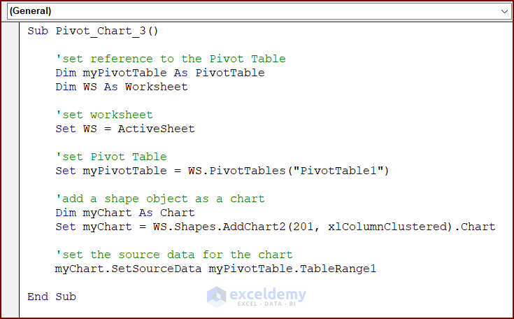
Method 3 – Use the Shape Object
We can apply the following VBA code based on Excel VBA Shape Object to create a chart from Pivot Table.
- Paste the following code in your VBA Editor and press the Run button or F5 key to run the code:
Sub Pivot_Chart_3()
    'set reference to the Pivot Table
    Dim myPivotTable As PivotTable
    Dim WS As Worksheet
    'set worksheet
    Set WS = ActiveSheet
    'set Pivot Table
    Set myPivotTable = WS.PivotTables("PivotTable1")
    'add a shape object as a chart
    Dim myChart As Chart
    Set myChart = WS.Shapes.AddChart2(201, xlColumnClustered).Chart
    'set the source data for the chart to be the Pivot Table range
    myChart.SetSourceData myPivotTable.TableRange1
End Sub
VBA Breakdown
Sub Pivot_Chart_3()- This line starts a new subroutine named Pivot_Chart_3.
    Dim myPivotTable As PivotTable
Dim WS As Worksheet- This code section declares two variables: myPivotTable of type PivotTable and WS of type Worksheet. These variables will be used to store references to the pivot table and worksheet objects, respectively.
Set WS = ActiveSheet- Then, this line assigns the active worksheet to the variable WS. The ActiveSheet property returns the currently active worksheet.
Set myPivotTable = WS.PivotTables("PivotTable1")- This code assigns the pivot table named PivotTable1 in the worksheet to the variable myPivotTable. The PivotTables property of the worksheet returns a collection of all the pivot tables in that worksheet.
    Dim myChart As Chart
Set myChart = WS.Shapes.AddChart2(201, xlColumnClustered).Chart- This code section adds a new shape object as a chart to the worksheet using the Shapes.AddChart2 method. The 201 parameter represents the chart type, and xlColumnClustered represents the clustered column chart type. The resulting chart object is assigned to the variable myChart.
myChart.SetSourceData myPivotTable.TableRange1- This line of code sets the source data for the chart to be the range of the pivot table using the SetSourceData method. The TableRange1 property of the pivot table returns the entire range of the pivot table data.
End Sub- This line ends the subroutine.

Read More: Types of Pivot Charts in Excel
Use Excel VBA to Create an Animated Chart from a Pivot Table
We can apply the following VBA code to create an animated chart from Pivot Table.

- Paste the following code in your VBA Editor and press the Run button or F5 key to run the code:
Sub Animated_Chart()
    'variable declaration
    Dim animation_delay As String
    Dim nRow As Long, nCol As Long
    Dim myRng As Range, PivotRng As Range
    Dim myArr() As Variant
    Dim WS As Worksheet
    'screen update ON
    Application.ScreenUpdating = True
    'set worksheet
    Set WS = ActiveSheet
    'set values of variables from Pivot Table
    Set myRng = WS.Range("B5:E17")
    Set PivotRng = WS.Range("G5:J17")
    nRow = myRng.Rows.Count
    nCol = myRng.Columns.Count
    animation_delay = "00:00:01"
    'array resize
    ReDim myArr(1 To nRow, 1 To nCol)
    'take values from range of cells to an array
    For i = 1 To nRow
        For j = 1 To nCol
            myArr(i, j) = myRng.Cells(i, j)
        Next j
    Next i
    'define range of selection
    WS.Range("L4").Select
    ActiveSheet.Shapes.AddChart.Select
    'set the data source to be Pivot Table range
    ActiveChart.SetSourceData Source:=WS.Range("$G$5:$J$17")
    'declare the chart type
    ActiveChart.ChartType = xlColumnClustered
    'declare activation command
    ActiveSheet.ChartObjects(1).Activate
    ActiveSheet.ChartObjects(1).Cut
    'select the chart destination
    WS.Select
    ActiveSheet.Paste
    'return to the worksheet
    WS.Select
    Range("B4").Activate
    'show values in range and create animated column chart race
    For i = 1 To nRow
        For j = 1 To nCol
            PivotRng.Cells(i, j) = myArr(i, j)
            DoEvents
        Next j
        DoEvents
        Application.Wait (Now + TimeValue(animation_delay))
    Next i
End Sub
VBA Breakdown
Sub Animated_Chart()- This line defines a VBA subroutine called Animated_Chart.
   Dim animation_delay As String
    Dim nRow As Long, nCol As Long
    Dim myRng As Range, PivotRng As Range
    Dim myArr() As Variant
Dim WS As Worksheet- This section of code declares several variables including animation_delay as a string, nRow and nCol as Long, myRng and PivotRng as Range, myArr as a dynamic variant array, and WS as a Worksheet.
Application.ScreenUpdating = True- This turns on the screen updating feature of the application.
Set WS = ActiveSheet- It sets the WS variable to refer to the currently active worksheet.
    Set myRng = WS.Range("B5:E17")
Set PivotRng = WS.Range("G5:J17")- This code section sets the values of the myRng and PivotRng ranges to specific cell ranges on the worksheet.
    nRow = myRng.Rows.Count
nCol = myRng.Columns.Count- This code section assigns the number of rows and columns in myRng to the nRow and nCol variables, respectively.
animation_delay = "00:00:01"- It sets the animation_delay variable to the value 00:00:01.
ReDim myArr(1 To nRow, 1 To nCol)- It resizes the myArr array to match the size of the myRng range.
    For i = 1 To nRow
        For j = 1 To nCol
            myArr(i, j) = myRng.Cells(i, j)
        Next j
Next i- This section of code uses a For loop and iterates through each value of myRng range. Then it copies the values from the myRng range to the corresponding element of myArr array.
    WS.Range("L4").Select
ActiveSheet.Shapes.AddChart.Select- It selects cell L4 on the worksheet and adds a chart object.
ActiveChart.SetSourceData Source:=WS.Range("$G$5:$J$17")- It sets the data source of the active chart to the PivotRng range.
ActiveChart.ChartType = xlColumnClustered- This line sets the chart type of the active chart to a clustered column chart.
    ActiveSheet.ChartObjects(1).Activate
ActiveSheet.ChartObjects(1).Cut- Then, this code section activates and cuts the first chart object on the worksheet.
    WS.Select
ActiveSheet.Paste- It selects the worksheet and pastes the chart object.
  WS.Select
Range("B4").Activate- This line of code activates cell B4 of the worksheet.
  For i = 1 To nRow
        For j = 1 To nCol
            PivotRng.Cells(i, j) = myArr(i, j)
            DoEvents
        Next j
        DoEvents
        Application.Wait (Now + TimeValue(animation_delay))
Next i- These nested loops iterate through each cell in the PivotRng range and assign the corresponding value from the myArr array. The DoEvents statement allows the operating system to process any pending events, and Application.Wait introduces a delay specified by animation_delay. This loop creates an animated effect by gradually updating the values in the range, simulating an animated column chart race.
End Sub- This line marks the end of the subroutine.
This code sets up an animated column chart race based on values from a Pivot Table. It copies a chart object, pastes it onto the worksheet, and then updates the values in a range over time to create an animated visualization.
Excel VBA Create a Pie Chart from a Pivot Table
We can use the following VBA code to create a Pie Chart from Pivot Table.

- Paste the following code in your VBA Editor and press the Run button or F5 key to run the code:
Sub Pie_Chart()
    'variable declaration
    Dim myCh As Chart
    Dim myPT As PivotTable
    Dim myPF As PivotField
    Dim WS As Worksheet
    'set worksheet
    Set WS = ActiveSheet
    'set pivot table
    Set myPT = WS.PivotTables(1)
    'add a chart
    Set myCh = Charts.Add
    'create a pie chart
    myCh.ChartType = xlPie
    'set the source data for the chart to be the Pivot Table range
    Set myPF = myPT.DataFields(1)
    myCh.SetSourceData myPT.TableRange1.Columns(myPF.DataRange.Column)
    'set the chart location
    myCh.Location Where:=xlLocationAsObject, Name:=WS.Name
End Sub
VBA Breakdown
Sub Pie_Chart()- This line defines a new subroutine named Pie_Chart.
    Dim myCh As Chart
    Dim myPT As PivotTable
    Dim myPF As PivotField
Dim WS As Worksheet- This section begins by declaring variables for different objects that will be used throughout the code. These variables include myCh of the Chart type, myPT of PivotTable type, myPF of the PivotField type, and WS of the Worksheet type.
Set WS = ActiveSheet- Then, this line sets the WS variable to the active sheet. This means that the code will work with the currently selected worksheet.
Set myPT = WS.PivotTables(1)- This code sets the value of myPT variable to the first PivotTable in the active sheet. This assumes that there is at least one PivotTable present.
Set myCh = Charts.Add- A new chart is added using the Charts.Add method. The newly created chart is assigned to the myCh variable.
    myCh.ChartType = xlPie
    Set myPF = myPT.DataFields(1)
myCh.SetSourceData myPT.TableRange1.Columns(myPF.DataRange.Column)\- The chart type is set to a pie chart using the xlPie constant. The source data for the chart is set to the data range of the first data field (myPF) in the Pivot Table (myPT). This ensures that the chart will display data from the PivotTable.
myCh.Location Where:=xlLocationAsObject, Name:=WS.Name- The chart is positioned in the worksheet specified by the WS object. The Location property is set to xlLocationAsObject to indicate that the chart should be placed as an object. The Name property is set to WS.Name to specify the name of the worksheet.
End Sub- This line marks the end of the subroutine.
Overall, the code declares variables, sets the worksheet and Pivot Table, creates a chart, configures it as a pie chart with the data from the pivot table, and positions the chart in the specified worksheet.

This pie chart is for the Asia region. You can change the region from the Region drop-down.
Read More: How to Refresh Pivot Chart in Excel
Things to Remember
There are a few things to remember while using Excel VBA to create a chart from Pivot Table:
- Specify the source data for the chart properly.
- Select the appropriate chart type.
- Indicate the chart location in the VBA code.
Frequently Asked Question
How do I determine the chart type?
To determine the chart type, you need to consider the nature of the data and the purpose of the chart. Excel provides various chart types such as column charts, bar charts, line charts, pie charts, etc.
Can I create the chart in a separate sheet?
Yes, you can create the chart in a separate chart sheet by using the Location property of the chart object.
How do I customize the appearance of the chart?
To customize the appearance of the chart, you can modify various chart properties such as titles, axis labels, legends, colors, and formatting. Use the properties and methods available on the chart object to make the desired adjustments.
Download the Practice Workbook
You can download this practice book while going through the article.
Related Articles
- Data Labels in Excel Pivot Chart
- Difference Between Pivot Table and Pivot Chart in Excel
- How to Edit Pivot Chart in Excel

