It does not always happen that you edit something in a place and it gets fixed automatically in all other places. But in Pivot Chart, we actually can do it. We can edit a thing in a dataset and it will get updated in the Pivot Chart by refreshing the Pivot Chart. In this article, I am going to explain 4 possible approaches to refresh the Pivot Chart in Excel. I hope it may help a little bit for Excel users.
Creating Excel Pivot Chart
In order to explain the refresh of the Pivot Chart in Excel, first of all, I am going to explain how to make a Pivot Chart. The steps are listed below.
Steps:
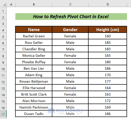
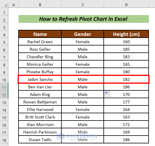
- Firstly, gather a dataset to create a Pivot Table which leads to a Pivot Chart. I have gathered data and decorated them in Name, Gender, and Height (cm) columns.
- Next, select all the data (i.e. B4:D17).
- Then, go to the Insert tab.
- Click on Pivot Table from the ribbon.
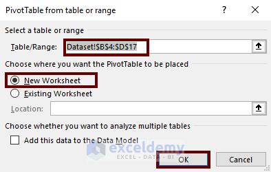
- Pick the From Table/Range option.

- Choose the pivot table location. I have selected the New Worksheet for the pivot table.
- Then, press the OK button.
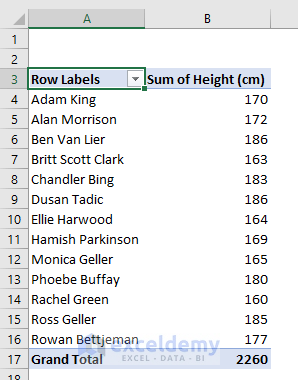
- From the Pivot Table Fields, pick rows and values. I have picked Name as Rows and Height as Values.

Then, we will have a default Pivot Table.
- We can edit the table according to our choice.
- Followingly, select all the cells in the Pivot Table.
- Go to the Insert tab.
- Choose Recommended Charts from the ribbon.

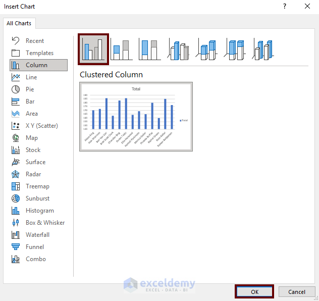
An Insert Chart wizard will appear.
- Select your chart type.
- Finally, press OK to have the Pivot Chart.
Thus, we can have a Pivot Chart.

Read More: How to Create Chart from Pivot Table in Excel
How to Refresh Pivot Chart in Excel: 4 Suitable Approaches
1. Refresh Manually from PivotChart Analyze
We can manually refresh the Pivot Chart from the PivotChart Analyze tab. It is the easiest way to refresh the Pivot Chart.
Steps:
- Update your dataset. In my case, I have added a whole new row with detailed information.
- Then, go to the PivotTable Analyze tab.
- Click on Refresh from the ribbon.

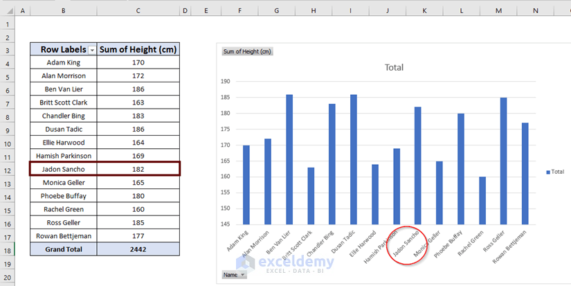
We will have the updated values both in the Pivot Table and Pivot Chart.
Read More: How to Edit Pivot Chart in Excel
2. Check Refresh Data When Opening File Option
Checking the Refresh data when opening the file box is another way to refresh the Pivot Chart.
Steps:
- Right-click on the Pivot Table.
- Select PivotTable Options…

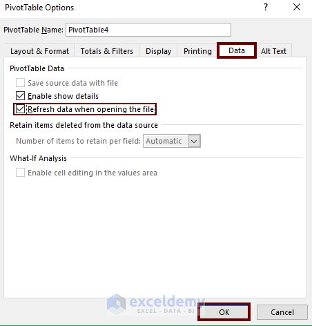
A Pivot Table Options box will appear.
- Click on the Data tab.
- Now, check the Refresh data when opening the file box.
We will have the refreshed Pivot Chart when opening the file.

Read More: Use Excel VBA to Create Chart from Pivot Table
3. Right-Click on Mouse to Refresh Pivot Chart
Another simple way to refresh Pivot Chart is to choose the Refresh option after right-clicking on the Pivot Table.
Steps:
- Put the cursor on the Pivot Table.
- Right-click on the mouse.
- Select Refresh from the available options.
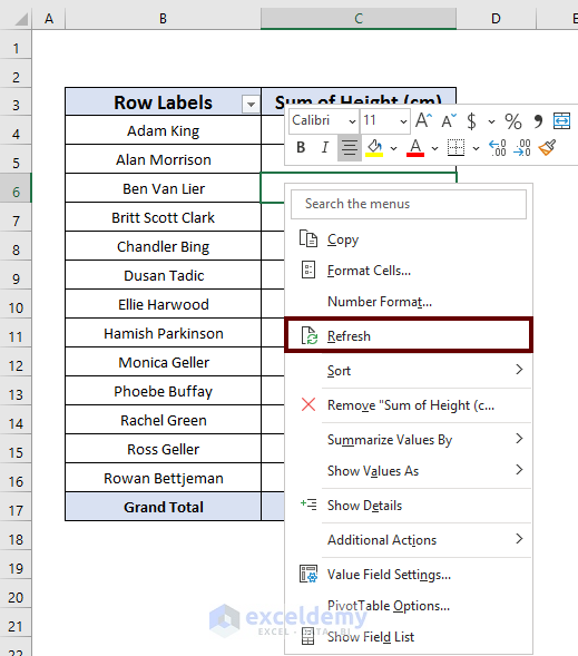
The Pivot Chart will be refreshed.

4. Using VBA to Refresh Pivot Chart
Using VBA is the smartest way to refresh Pivot Chart.
Steps:
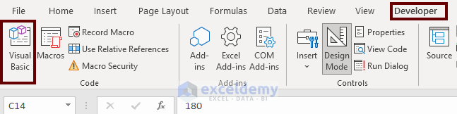
- Firstly, go to the Developer tab.
- Then, pick Visual Basic from the ribbon.
- Double-click on the Sheet to have the space to write the code.

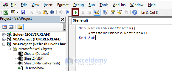
- Insert the following code.
Sub RefreshPivotCharts()
     ActiveWorkbook.RefreshAll
End Sub
Here, I have a Sub_procedure named RefreshPivotCharts. I have applied ActiveWorkbook.RefreshAll properties to automatically update the Pivot Chart.
- Click on the Run or F5 button.
This is another cool way to refresh the pivot chart.

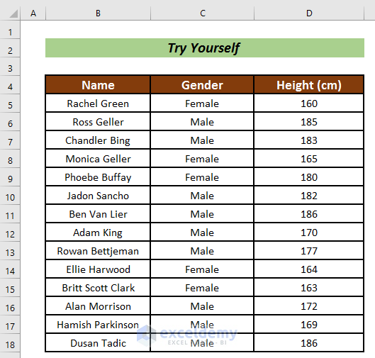
Practice Section
You can practice here for further expertise.
Download Practice Workbook
Conclusion
That’s all for the article. In this article, I have tried to explain 4 possible approaches to refresh the Pivot Chart in Excel. It will be a matter of great pleasure for me if this article could help any Excel user even a little. For any further queries, comment below.
Related Articles
- How to Use Pivot Chart in Excel
- Types of Pivot Charts in Excel
- Data Labels in Excel Pivot Chart
- Difference Between Pivot Table and Pivot Chart in Excel

