How to Statistically Analyze Data in Excel (5 Ways)

Method 1 – Calculating Central Tendency and Variability

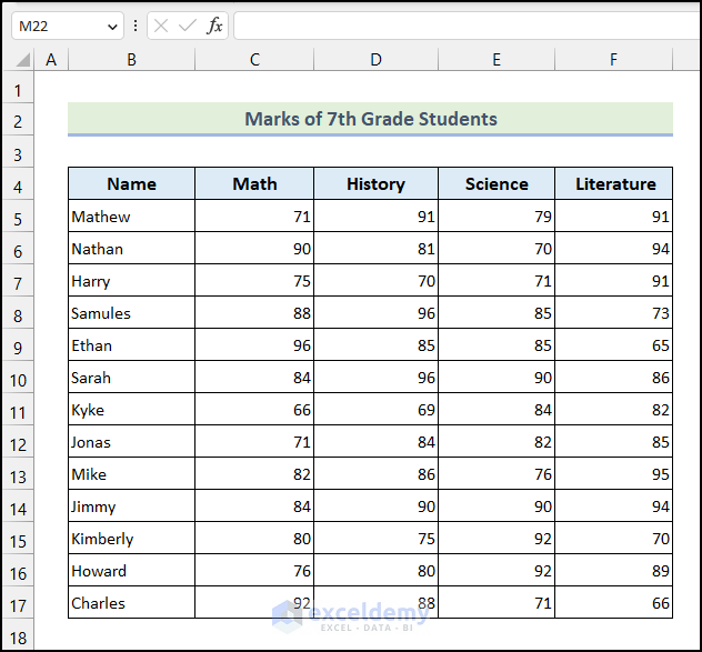
The above dataset marks of 7th-grade students are given based on Math, History, Science, and Literature subjects.

1.1 Using the AVERAGE Function

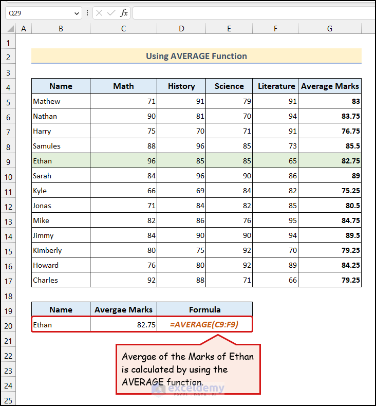
You see the Average Marks for Ethan in cell C20.

Here, we have used the AVERAGE function, which returns the arithmetic mean of a dataset.

• Enter the following formula in cell C20:

1.2 Employing AVERAGEIF and AVERAGEIFS Functions

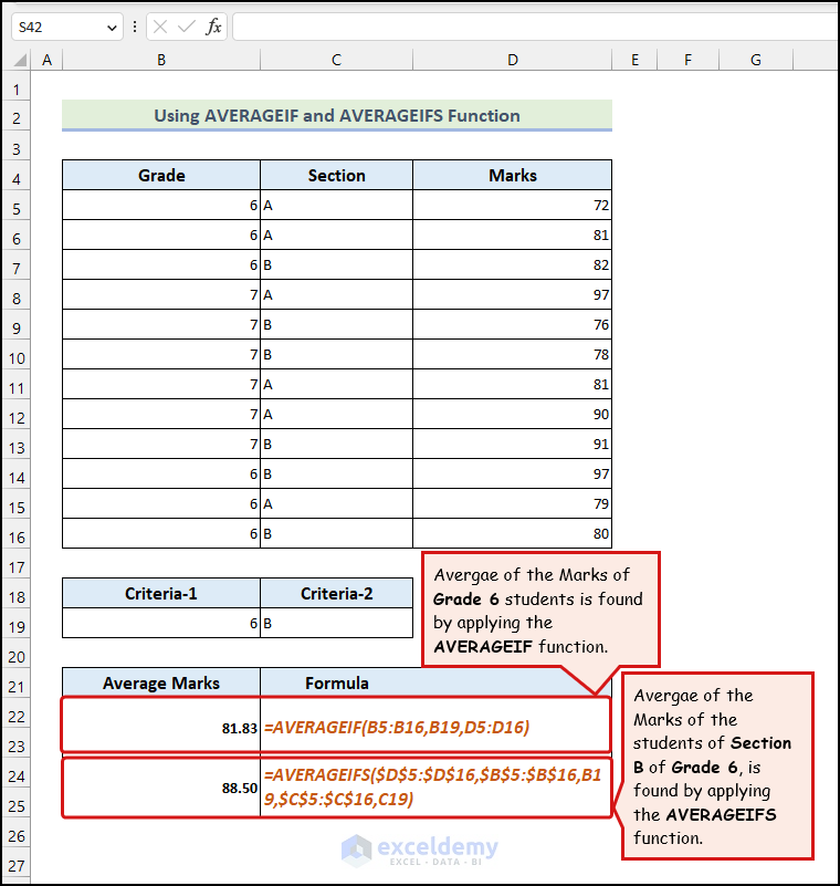
The above dataset demonstrates the diverse uses of the AVERAGEIF and AVERAGEIFS functions.

You want to find the average of the marks obtained by the Grade 6 students. To do this,

• Enter the following formula in cell B22:

Let’s assume another situation where we want to find the Average Marks of the students based on two criteria: their Grade and Section.

• Enter the following formula in cell C24:

1.3 Utilizing HARMEAN and GEOMEAN Functions

Let’s say we have six numbers as our data. The numbers are 1,2,3,4,5 and 6. Then our harmonic mean value will be as follows.

The GEOMEAN function calculates the Geometric Mean of a selected dataset. The geometric mean is calculated by finding the nth root after multiplying the n values of a dataset. Here, n is the total number of values in a dataset. For instance, let’s say we have 5 numbers as our dataset. These are 1, 2, 3, 4, and 5. So, the Geometric Mean will be,

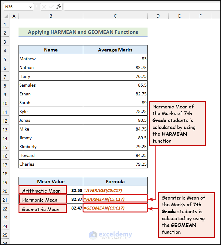
The above image demonstrates a practical example of using both HARMEAN and GEOMEAN functions.

• The formula for calculating the harmonic mean in the B21 cell is:

One thing is clear: the value of the harmonic mean, in this case, is lower than the average value of the Average Marks. The arithmetic mean is 82.58, but the harmonic mean is 82.37. That means it limits the value of the large value of Average Marks.

• In the case of finding the geometric mean, we have used the following formula in cell C22:

Like the harmonic mean, the geometric mean (82.47) differs from the arithmetic mean (82.58). Investors use the geometric mean as it provides a more accurate average value whenever row values are given across several periods.

1.4 Applying STANDARDIZE Function

Steps:

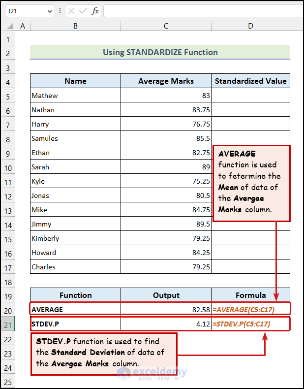
• Calculate the Mean and the Standard Deviation of the dataset.

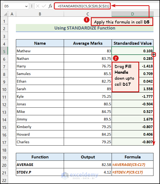
• Enter the following formula in cell D5:

You can use the MODE.SNGL, MEDIAN, VAR.S, VAR.P, STDEV.S, and STDEV.P functions to further statistically analyze data in Excel.

Method 2 – Computing Relative Standing

Let’s say both the 5th and 6th-ranked values are the same. In that case, the RANK.EQ function will return rank 5 for both values, and the next rank value will be rank 7. Here, we have the Total Marks of 7th Grade Students as our dataset.

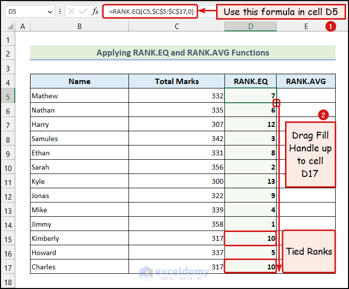
Here, you can see that the 10th and the 11th values were tied. So, the RANK.EQ function returned rank 10 for both values.

• We have applied the following formula in cell D5.

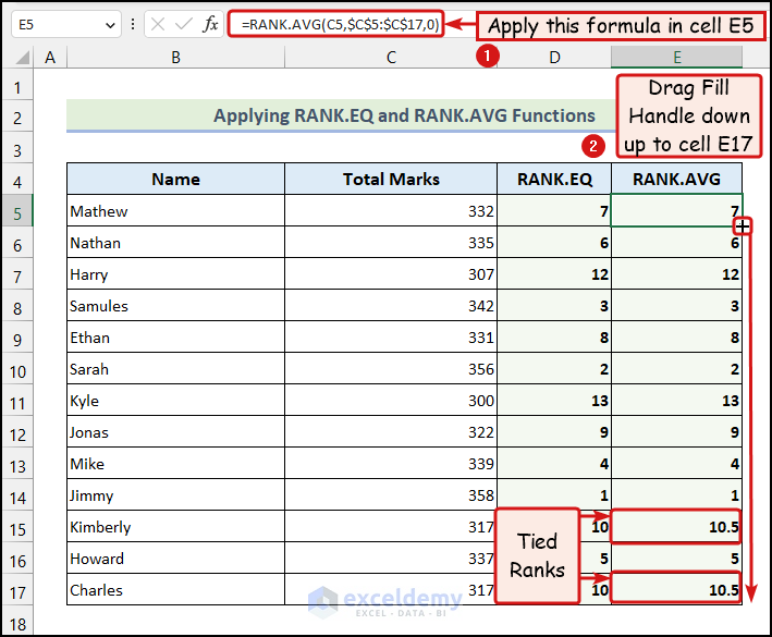
Here, the 10th and 11th values were tied, so the RANK.AVG function returned an average of 10.5 for both values.

The RANK.AVG function also returns the relative ranks of a dataset. But, in the case of ties, it will return an average rank for the tied values. For example, let’s say the 4th and 5th-ranked values are tied. So, the RANK.AVG function will return a rank of 4.5 for both values. The rank of the next value will be 6. Now, let’s use the instructions outlined below to utilize the RANK.AVG function in Excel to statistically analyze data.

• We have used the following formula in cell E5:

Furthermore, you can also use the PERCENTRANK.INC, PERCENTRANK.EXC, PERCENTILE.INC, PERCENTILE.EXC, QUARTILE.INC and QUARTILE.EXC functions to compute the relative standing of data in Excel.

Method 3 – Determining Correlation and Regression

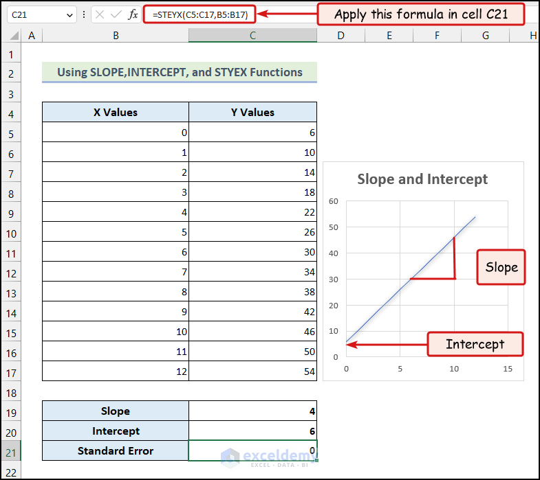
3.1 Using SLOPE, INTERCEPT, and STYEX Functions

The STYEX function gives us the standard error of Y Values for given X Values. We can use it to predict the Y Value from an X Value.

Steps:

• Enter the formula given below in cell C21:

• Press ENTER.

You will have the Standard Error of the Y Values for given X Values in cell C21.

3.2 Applying CORREL Function

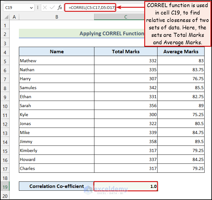
The CORREL function helps us find how closely two sets of data are related.

• We have used the following formula in the C19 cell:

4. Applying Array Functions for Statistical Analysis

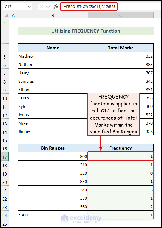
Here, we have the frequencies against each Bin Range, as demonstrated in the following picture. We have used the FREQUENCY function, one of the most commonly used array functions, to analyze data in Excel statistically.

• Enter the following formula in cell C17:

You can use the MODE.MULT function, LINEST function, TREND function, and GROWTH function to statistically analyze data in Excel.

Note: If you are using an older version of Excel, you might need to press CTRL + SHIFT + ENTER to use the array formulas. As we use Excel 365, simply pressing ENTER will do for us.

Method 5 – Utilizing Data Analysis ToolPak to Calculate Moving Average

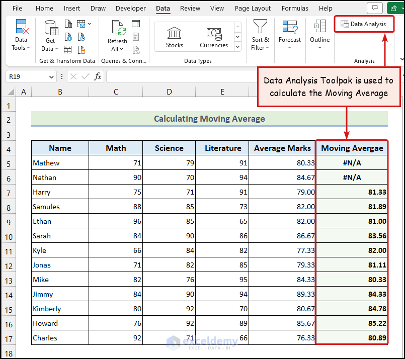
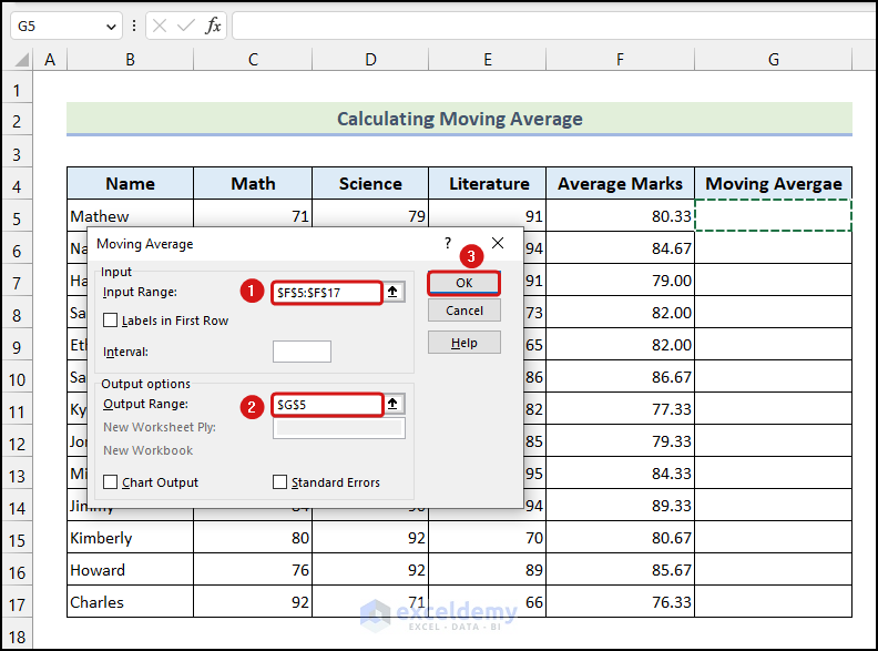
The above image represents the Moving Average of our dataset. The Data Analysis ToolPak option is not in the Excel Ribbon by default. You will need to activate this feature manually. You can follow this article to activate the Data Analysis ToolPak and also learn about its various uses.

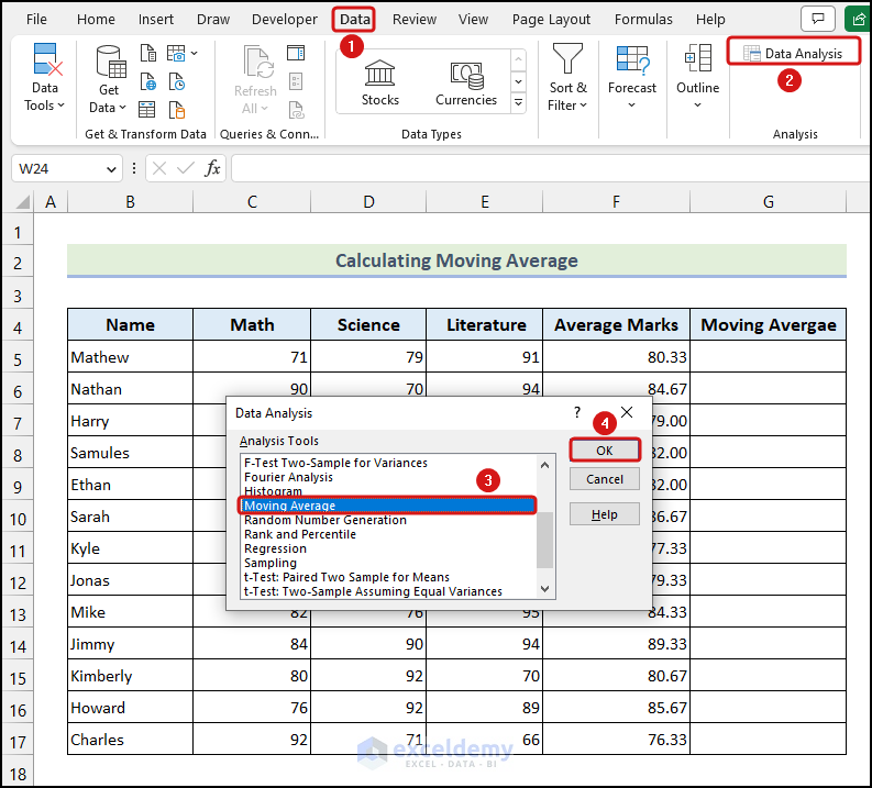
• Go to the Data tab from Ribbon >> choose the Data Analysis option from the Analysis group.

The Data Analysis dialogue box will appear on your worksheet, as shown in the above image.

• Go to the Input Range field to select the cells of the Average Marks column >> click on the Output Range field and select cell G5 >> click OK.

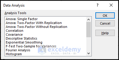
Some Common Data Analysis Tools in Excel

• Anova: Single Factor → It analyzes variance for two or more observations.
• Anova: Two Factor with Replication → For each combination of the variables’ levels, it creates an analysis of variance with two independent variables and various observations.
• Anova: Two Factor Without Replication → For each combination of the variables’ levels, it creates an analysis of variance with two independent variables and a single observation.
• Correlation → When there are more than two measurements on a sample of people, a matrix of correlation coefficients for each possible pair of measurements is computed.
• Covariance → When there are more than two measurements on a sample of people, a matrix of covariance coefficients is computed for each possible pair of measurements.
• Descriptive Statistics → It produces a report summarizing the central tendency, variability, and other properties of values within a defined range of cells.
• Exponential Smoothing → It predicts the next value of a sequence, using the sequence of the previous values and previous predictions.
• F-Test Two-Sample for Variances → It compares two variances by performing an F-Test.
• Histogram → It builds a tabular depiction of the frequency distribution of values within a chosen cell range.
• Random Number Generation → Based on one of the seven potential distributions, generates a specific quantity of random numbers.
• Rank and Percentile → It creates a table displaying each value in a set of values along with its ordinal and percentile ranks.
• Regression → This creates a report of the linear regression statistics applied to a set of data that includes one dependent variable and one or more independent variables.
• Sampling → It generates a sample of values from the cells in the specified range.

You’ll get the following analysis tools in the Data Analysis ToolPak.

Things to Remember

• Before performing any data analysis in Excel, you must be clear about your data type, e.g., continuous or categorical.
• Next, you must select from the enriched list of statistical analysis tools, such as t-test, ANOVA, regression, and correlation.
• Once you’ve conducted your analysis, it’s important to interpret your results meaningfully. This means understanding what the numbers mean and how they relate to your research question.
• Finally, validating your results by checking for errors and ensuring that your analysis is robust is important. This includes checking for outliers, testing assumptions, and conducting sensitivity analyses.

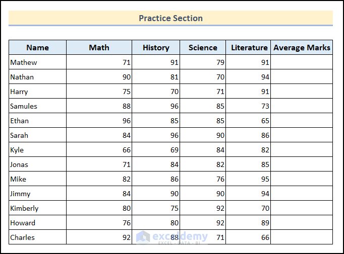
Practice Section

In the Excel Workbook, we have provided a Practice Section on the right side of the worksheet.

A sample practice section is provided in each worksheet of the Practice Workbook.

Download the Practice Workbook

Download the following workbook and practice.