This tutorial will demonstrate how to make a calendar in Excel without a template. In our day-to-day life, we all use a deadline for certain work or projects, so it is very important to maintain our own calendar. It helps you in reminding your work time limits. Moreover, creating your own Excel calendar can give you an extra edge as you can modify it as you desire. So, it is very important to make a calendar in Excel without a template.
Make a Calendar in Excel Without Template: 2 Easy Examples
We will use 2 examples to make a calendar in Excel without a template. If you follow the steps correctly, you should learn how to make a calendar in Excel without a template on your own. The steps are:
1. Creating Monthly Calendar in Excel
In this case, our goal is to create a monthly calendar without using any template. We can easily do that by following the steps below.
Steps:
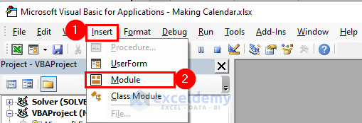
- First, press the Alt + F11 options to open the VBA window.
- Then, go to the Insert > Module options.
- After that, insert the following code in the window.
Sub CalendarMaker()
'This code was taken from extendoffice.com
       ActiveSheet.Protect DrawingObjects:=False, Contents:=False, _
          Scenarios:=False
       Application.ScreenUpdating = False
       On Error GoTo MyErrorTrap
       Range("a1:g14").Clear
       MyInput = InputBox("Type in Month and year for Calendar ")
       If MyInput = "" Then Exit Sub
       StartDay = DateValue(MyInput)
       If Day(StartDay) <> 1 Then
           StartDay = DateValue(Month(StartDay) & "/1/" & _
               Year(StartDay))
       End If
       Range("a1").NumberFormat = "mmmm yyyy"
       With Range("a1:g1")
           .HorizontalAlignment = xlCenterAcrossSelection
           .VerticalAlignment = xlCenter
           .Font.Size = 18
           .Font.Bold = True
           .RowHeight = 35
       End With
       With Range("a2:g2")
           .ColumnWidth = 11
           .VerticalAlignment = xlCenter
           .HorizontalAlignment = xlCenter
           .VerticalAlignment = xlCenter
           .Orientation = xlHorizontal
           .Font.Size = 12
           .Font.Bold = True
           .RowHeight = 20
       End With
       Range("a2") = "Sunday"
       Range("b2") = "Monday"
       Range("c2") = "Tuesday"
       Range("d2") = "Wednesday"
       Range("e2") = "Thursday"
       Range("f2") = "Friday"
       Range("g2") = "Saturday"
       With Range("a3:g8")
           .HorizontalAlignment = xlRight
           .VerticalAlignment = xlTop
           .Font.Size = 18
           .Font.Bold = True
           .RowHeight = 21
       End With
       Range("a1").Value = Application.Text(MyInput, "mmmm yyyy")
       DayofWeek = Weekday(StartDay)
       CurYear = Year(StartDay)
       CurMonth = Month(StartDay)
       FinalDay = DateSerial(CurYear, CurMonth + 1, 1)
       Select Case DayofWeek
           Case 1
               Range("a3").Value = 1
           Case 2
               Range("b3").Value = 1
           Case 3
               Range("c3").Value = 1
           Case 4
               Range("d3").Value = 1
           Case 5
               Range("e3").Value = 1
           Case 6
               Range("f3").Value = 1
           Case 7
               Range("g3").Value = 1
       End Select
       For Each cell In Range("a3:g8")
           RowCell = cell.Row
           ColCell = cell.Column
           If cell.Column = 1 And cell.Row = 3 Then
           ElseIf cell.Column <> 1 Then
               If cell.Offset(0, -1).Value >= 1 Then
                   cell.Value = cell.Offset(0, -1).Value + 1
                   If cell.Value > (FinalDay - StartDay) Then
                       cell.Value = ""
                       Exit For
                   End If
               End If
           ElseIf cell.Row > 3 And cell.Column = 1 Then
               cell.Value = cell.Offset(-1, 6).Value + 1
               If cell.Value > (FinalDay - StartDay) Then
                   cell.Value = ""
                   Exit For
               End If
           End If
       Next
       For x = 0 To 5
           Range("A4").Offset(x * 2, 0).EntireRow.Insert
           With Range("A4:G4").Offset(x * 2, 0)
               .RowHeight = 65
               .HorizontalAlignment = xlCenter
               .VerticalAlignment = xlTop
               .WrapText = True
               .Font.Size = 10
               .Font.Bold = False
               .Locked = False
           End With
           With Range("A3").Offset(x * 2, 0).Resize(2, _
           7).Borders(xlLeft)
               .Weight = xlThick
               .ColorIndex = xlAutomatic
           End With
           With Range("A3").Offset(x * 2, 0).Resize(2, _
           7).Borders(xlRight)
               .Weight = xlThick
               .ColorIndex = xlAutomatic
           End With
           Range("A3").Offset(x * 2, 0).Resize(2, 7).BorderAround _
              Weight:=xlThick, ColorIndex:=xlAutomatic
       Next
       If Range("A13").Value = "" Then Range("A13").Offset(0, 0) _
          .Resize(2, 8).EntireRow.Delete
       ActiveWindow.DisplayGridlines = False
       ActiveSheet.Protect DrawingObjects:=True, Contents:=True, _
          Scenarios:=True
       ActiveWindow.WindowState = xlMaximized
       ActiveWindow.ScrollRow = 1
       Application.ScreenUpdating = True
       Exit Sub
MyErrorTrap:
       MsgBox "You may not have entered your Month and Year correctly." _
           & Chr(13) & "Spell the Month correctly" _
           & " (or use 3 letter abbreviation)" _
           & Chr(13) & "and 4 digits for the Year"
       MyInput = InputBox("Type in Month and year for Calendar")
       If MyInput = "" Then Exit Sub
       Resume
   End Sub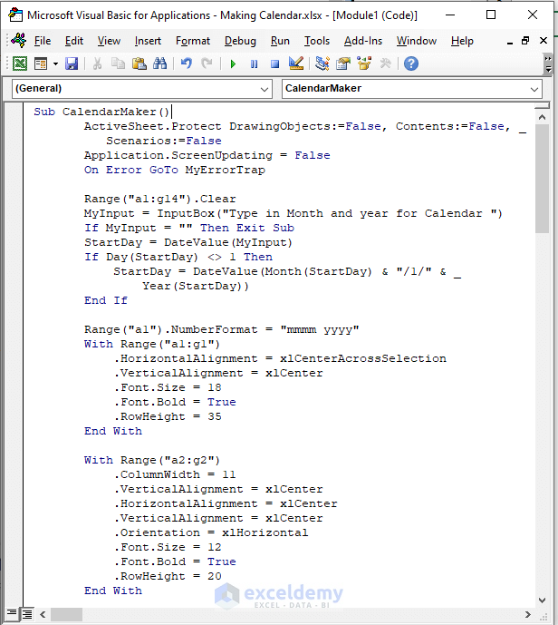
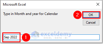
- Next, insert the desired month and year in the calendar dialog box and press OK.
- Finally, after pressing the RUN or F5 button, you will get the desired result.

Read More: How to Create a Monthly Calendar in Excel
2. Making Yearly Calendar in Excel
We want to create a yearly calendar in Excel by following the steps below.
Steps:
- First, arrange a dataset like the below image.


- Next, insert the following formula in cell B8.
=IF(MONTH(DATE($B$4,$B$6,1)+SEQUENCE(6,7)-WEEKDAY(DATE($B$4,$B$6,1),2))=$B$6,DATE($B$4,$B$6,1)+SEQUENCE(6,7)-WEEKDAY(DATE($B$4,$B$6,1),2),"")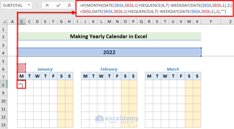
🔎 How Does the Formula Work?
- (DATE($B$4,$B$6,1): this portion represents the selected cells on which the DATE function will be applied.
- WEEKDAY(DATE($B$4,$B$6,1),2): this portion takes into consideration on date and weekday both together.
- (DATE($B$4,$B$6,1)+SEQUENCE(6,7)-WEEKDAY(DATE($B$4,$B$6,1),2))=$B$6,DATE($B$4,$B$6,1)+SEQUENCE(6,7)-WEEKDAY(DATE($B$4,$B$6,1),2): this portion represents that the dates are sequentially organized with the consideration of dates and weekdays.
- IF(MONTH(DATE($B$4,$B$6,1)+SEQUENCE(6,7)-WEEKDAY(DATE($B$4,$B$6,1),2))=$B$6,DATE($B$4,$B$6,1)+SEQUENCE(6,7)-WEEKDAY(DATE($B$4,$B$6,1),2),””): this portion represents the whole conditions along with months, dates and weekdays.
- Then, after pressing the Enter button, you will get the desired result for that month.

- After that, if you keep repeating the steps, you will get the desired result for every month of the year like the below image.


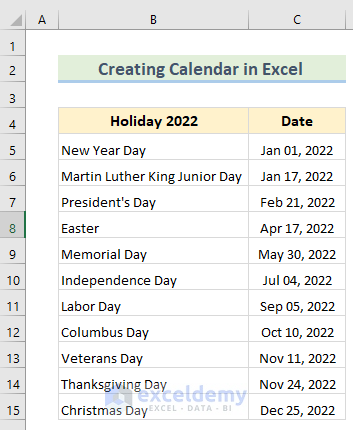
- Now, we want to insert the holidays into the current yearly calendar. So, we have arranged a dataset like the below image in the new worksheet.
- Next, go to the selected Data table > Home > Conditional Formatting > New Rules options.

- Then, in the New Formatting Rule dialog box, select the Use a formula to determine which cells to format in the Select a Rule Type option and insert the following rule in the Format values where this formula is a true option and select the desired color in the Preview option and press OK.
=ISNUMBER(VLOOKUP(B8,Holidays!$C:$C,1,0))
🔎 How Does the Formula Work?
- VLOOKUP(B8, Holidays!$C:$C,1,0): the VLOOKUP function looks for a value in the left-most column of a table, and then returns a value in the same row from a column you specify. Here, B6 (lookup_value argument) is mapped from the Holidays!$C:$C (table_array argument) array. Next, 1 (col_index_num argument) represents the column number of the lookup value. Lastly, 0 (range_lookup argument) refers to the Exact match of the lookup value.
- ISNUMBER(VLOOKUP(B8, Holidays!$C:$C,1,0)): the ISNUMBER function checks whether a value is a number and returns TRUE or FALSE.
- Next, after pressing the Enter button, you will get the desired result for that month.

- Last, if you keep repeating the steps, you will get the desired result for every month of the year like the below image.


Read More: How to Create a Yearly Calendar in Excel
Download Practice Workbook
You can download the practice workbook from here.
Conclusion
Henceforth, follow the above-described methods. Hopefully, these methods will help you to make a calendar in Excel without a template. We will be glad to know if you can execute the task in any other way. Please feel free to add comments, suggestions, or questions in the section below if you have any confusion or face any problems. We will try our level best to solve the problem or work with your suggestions.
Related Articles
- How to Create a Weekly Calendar in Excel
- How to Make an Interactive Calendar in Excel
- How to Make a Blank Calendar in Excel

