How to Make an Interactive Calendar in Excel (2 Easy Ways)

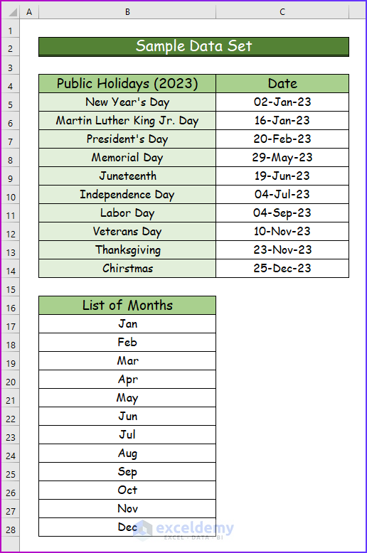
The sample dataset below will be used for illustration.

Method 1 – Making Interactive Monthly Calendar in Excel

Step 1:

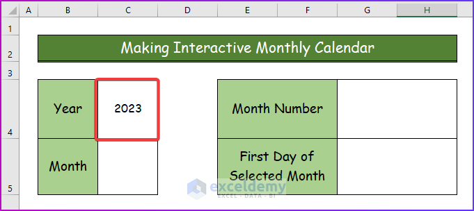
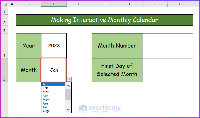
• Open a new sheet and create four fields for user inputs and name them.
• To create the monthly calendar for the year 2023, input that in the year field.

Step 2:

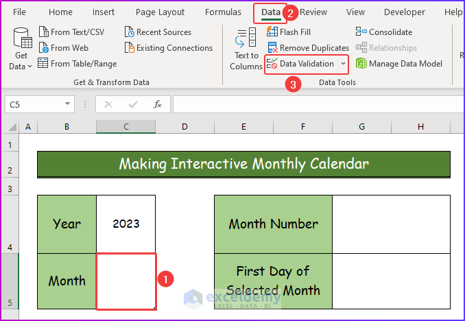
• Select cell C5 and go to the Data tab of the ribbon.
• From the Data Tools group, select Data Validation.

Step 3:

• Under the Allow dropdown select List and in the Source type box, select the data range of the twelve months.
• Press OK.

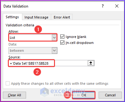
• This will create a dropdown of the twelve months in cell C5.

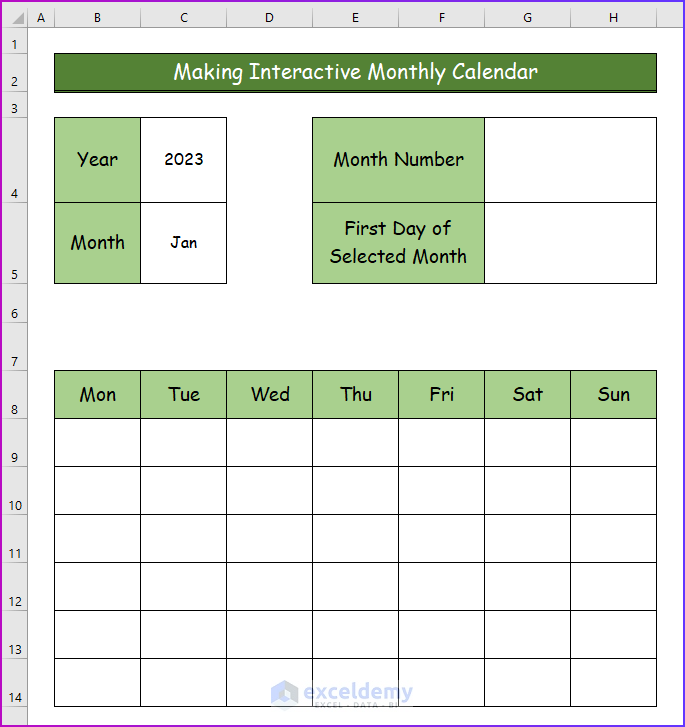
Step 4:

• Create a 7×7 table.
• Enter the day names of the week in the created table. Monday being in the first column.

Step 5:

• To make the header a dynamic one, join the cell values of C5 and C4 by entering the following formula.

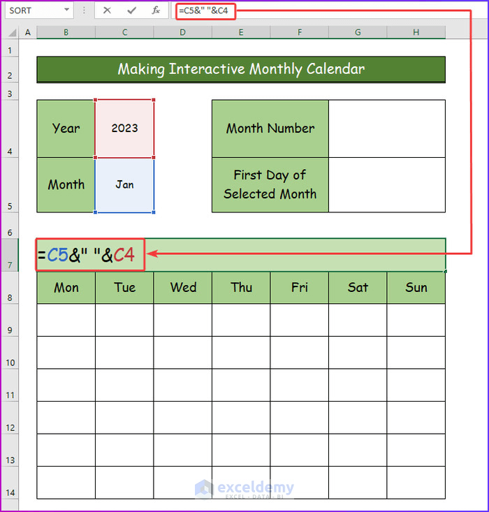
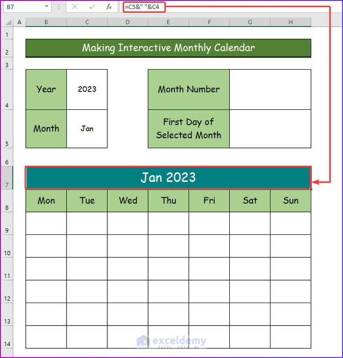
Step 6:

• The header will change to the values from cell C5 and C4.

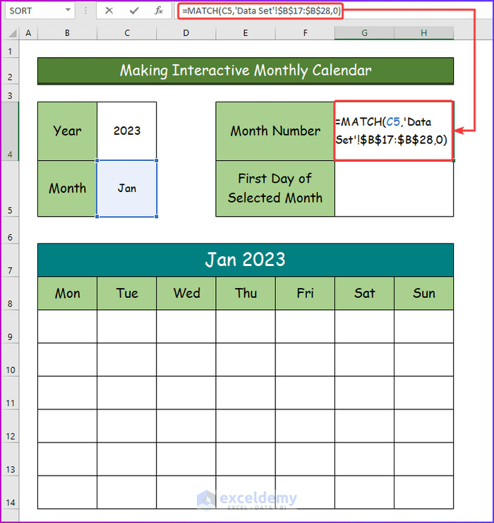
Step 7:

• Enter the the MATCH function in cell G4.

• The MATCH function will search the cell value of C5 in the B17:B28 cell range and will return the relative position of that month in that range.

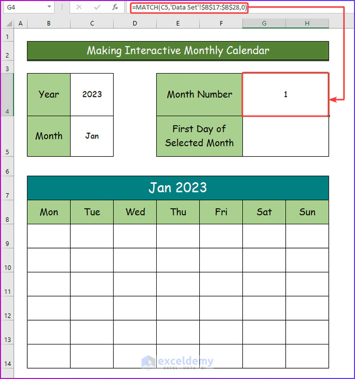
Step 8:

• Press Enter to find the month number of cell C5 in cell G4.

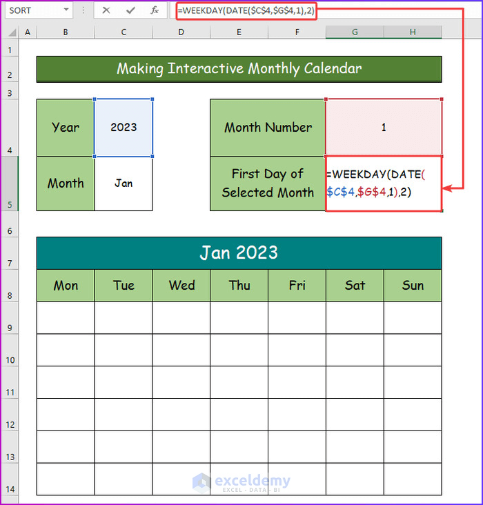
Step 9:

• Determine the first day for each month in a year in the form of a number.
• 1 will represent Monday, 2 will represent Tuesday etc.
• Insert the following combination formula of WEEKDAY and DATE functions in cell G5.

• The Date function will show the first date of each month of a specific year.
• The combination formula will return the first day for each month through the WEEKDAY function.
• Start the week from Monday. Enter 2 as the return type in the formula.

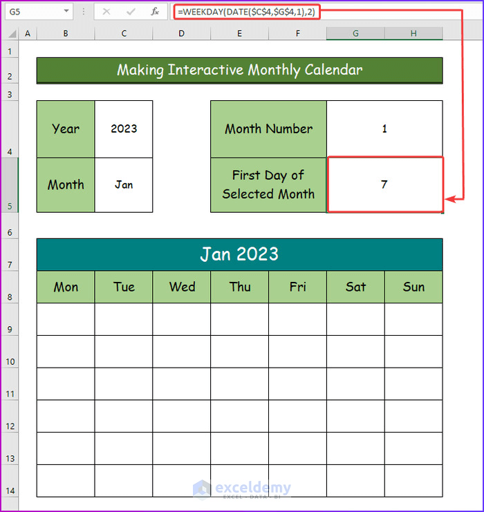
Step 10:

• The formula will show the number corresponding to the first day of January 2023 which is 7 and a Sunday.

Step 11:

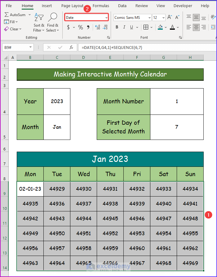
• To fill up the table with numbers, enter the following formula of the SEQUENCE function in cell B9.

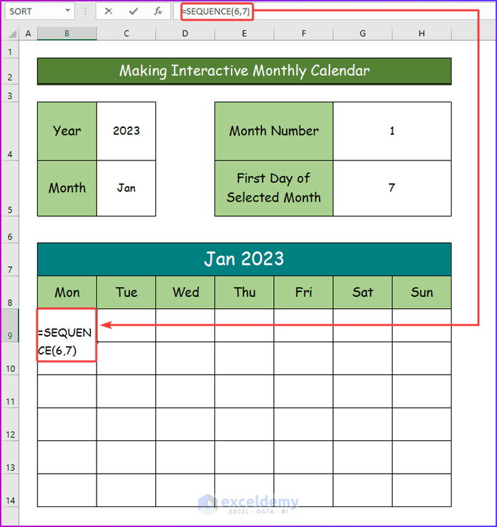
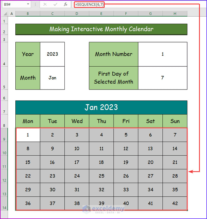
Step 12:

• There are 6 columns and 7 rows in the table. The table will fill up by numbers from 1-42 serially.

Step 13:

• To convert the numbers into dates, enter the following formula in cell B9.

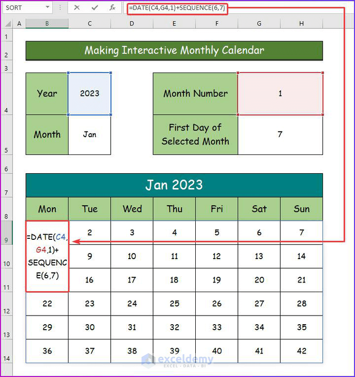
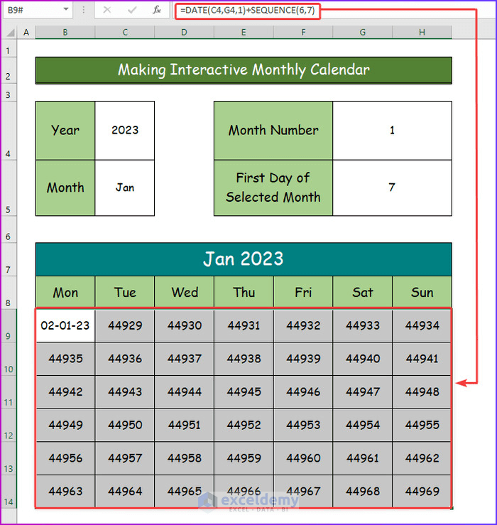
Step 14:

• Press Enter to get the result as shown in the image below.

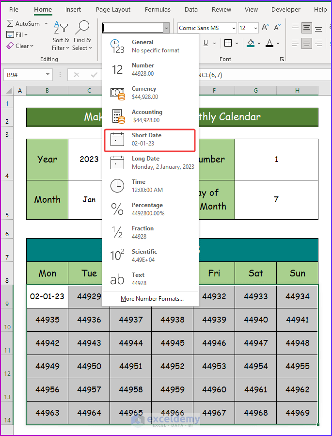
Step 15:

• The outputs are not in the correct format.
• To modify them, select the cell range B9: H14 and choose the Number Format dropdown in the Number group.

Step 16:

• Select Short Date as the format for the selected cell range.

Step 17:

• The starting date or day of Jan 2023 is not correct.

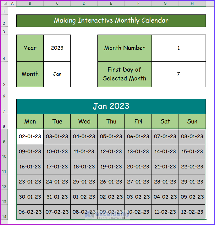
Step 18:

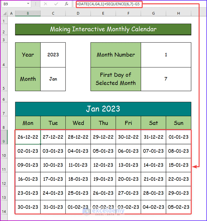
• To modify it, enter the following formula in cell B9:

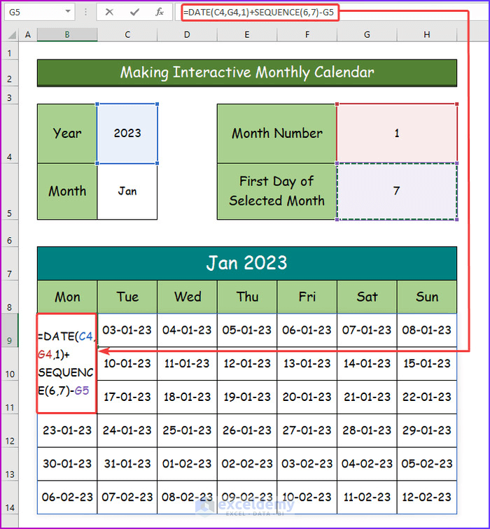
Step 19:

• The result shows the starting date for January as Sunday, as shown in the image below.
• There are some extra dates from the previous and following months of January 2023.

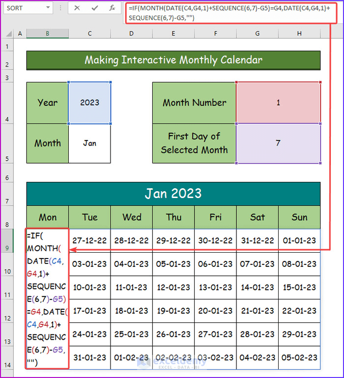
Step 20:

• Extract those extra days from the calendar by entering the following combination formula in cell B9.

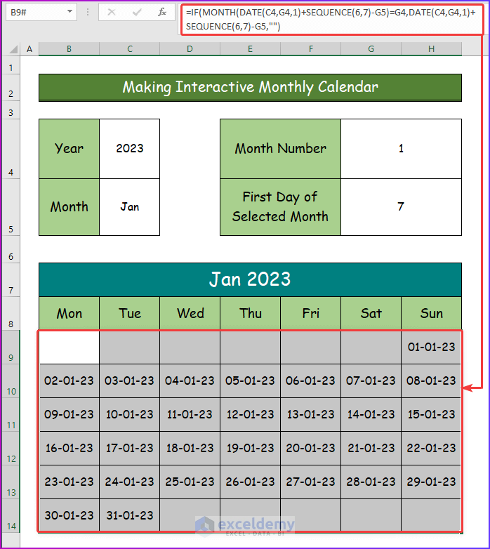
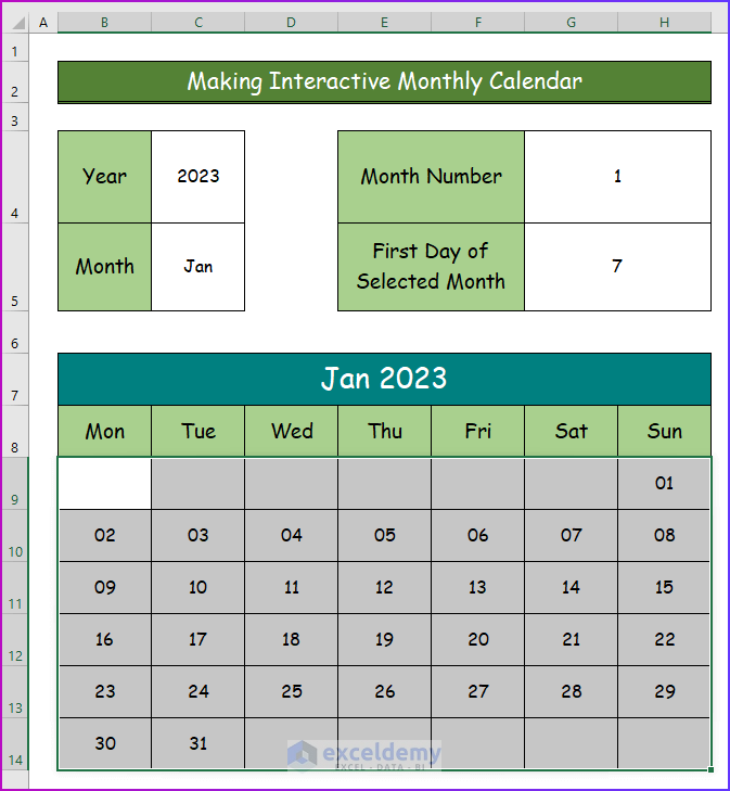
Step 21:

• The monthly calendar dates are updated correctly as shown in the image below.

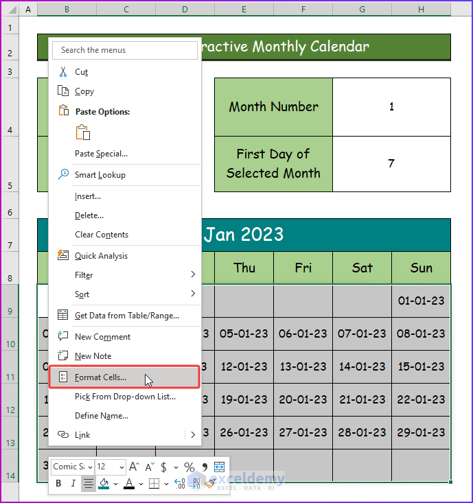
Step 22:

• Right-click on the mouse after selecting the data range B9:H14 to transform the format of dates.
• From the context, select Format Cells.

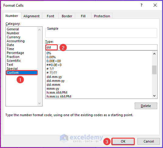
Step 23:

• The Format Cells dialog box will open.
• Go to the Custom tab in the dialog box.
• Under the Type label, type dd.
• Press OK.

Step 24:

• This keeps the dates in the table.

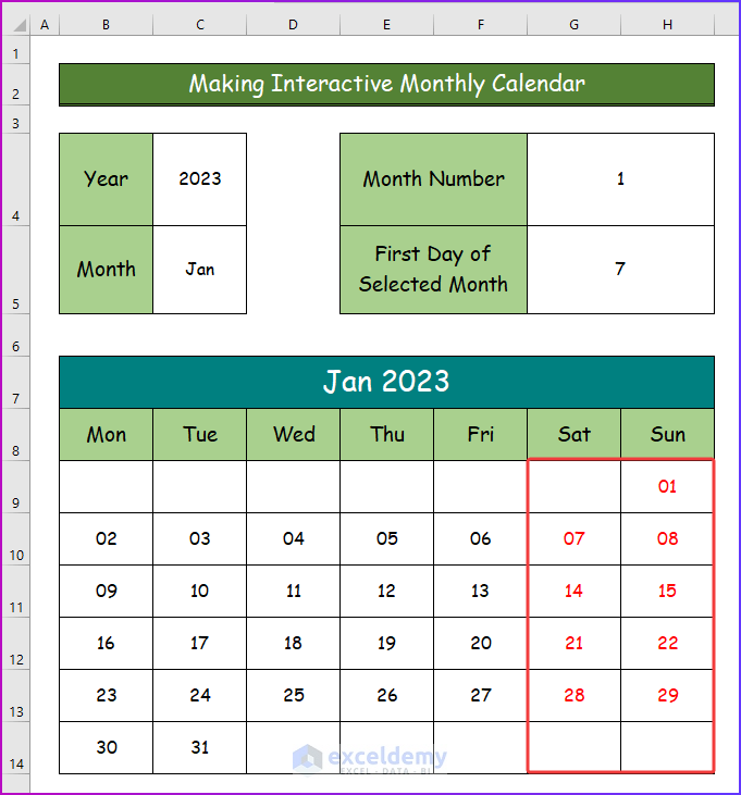
Step 25:

• Change the font color for the weekends from black to red.

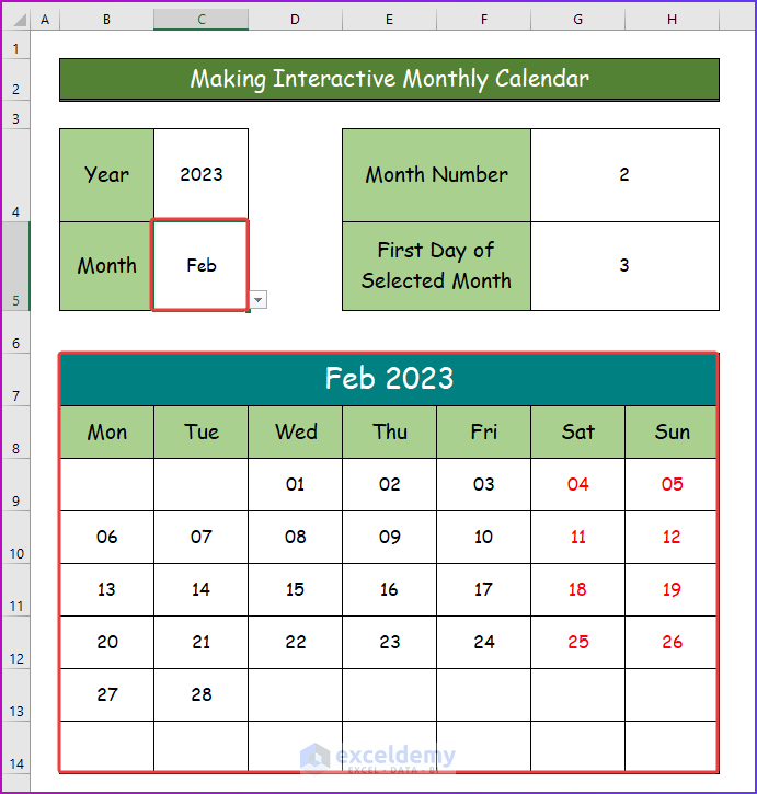
Step 26:

• When you change the month name from the dropdown in cell C5, the dates will also be changed in the data range of the monthly calendar.

Step 27:

• Select the cell range B5:H14 to highlight the holidays for each month.
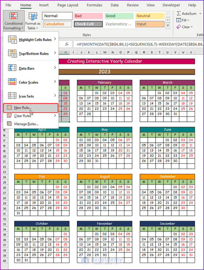
• Go to the Home tab of the ribbon and select Conditional Formatting.
• From the dropdown, choose New Rule.

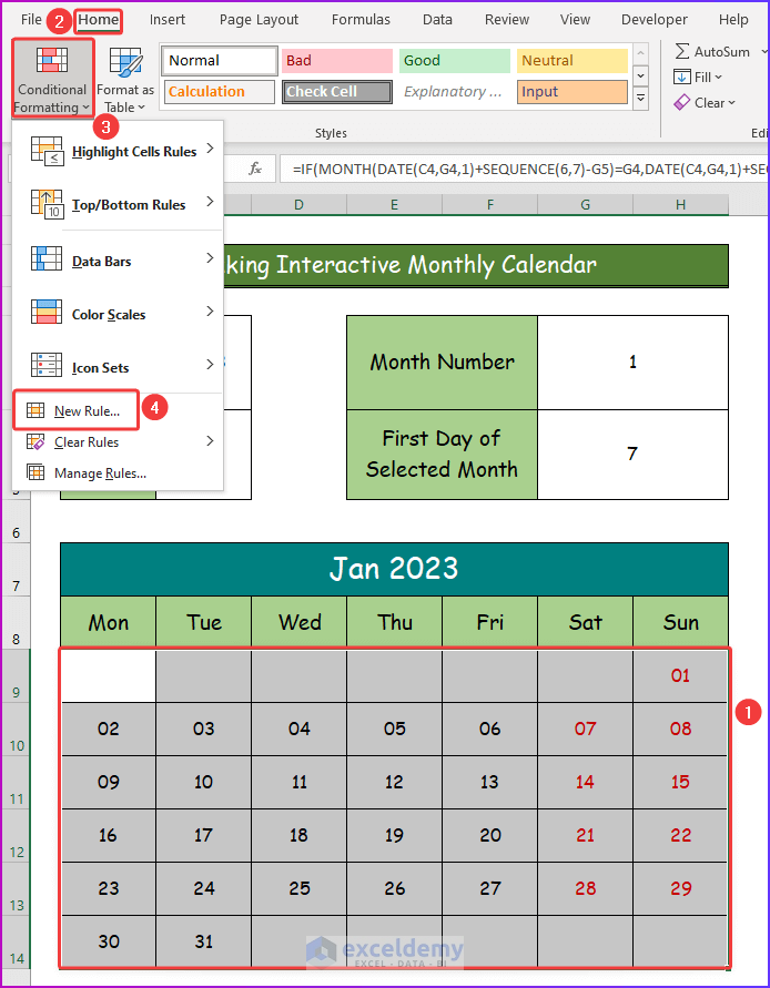
Step 28:

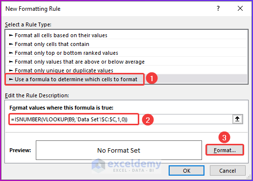
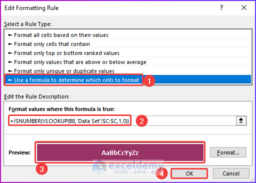
• The New Formatting Rule dialog box open.
• Under Select a Rule Type header, select Use a formula to determine which cells to format.
• Enter the following combination formula of ISNUMBER and VLOOKUP.

• Press Format to format the cells.

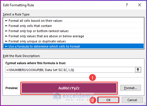
Step 29:

• Choose the desired color and font style and click OK.

Step 30:

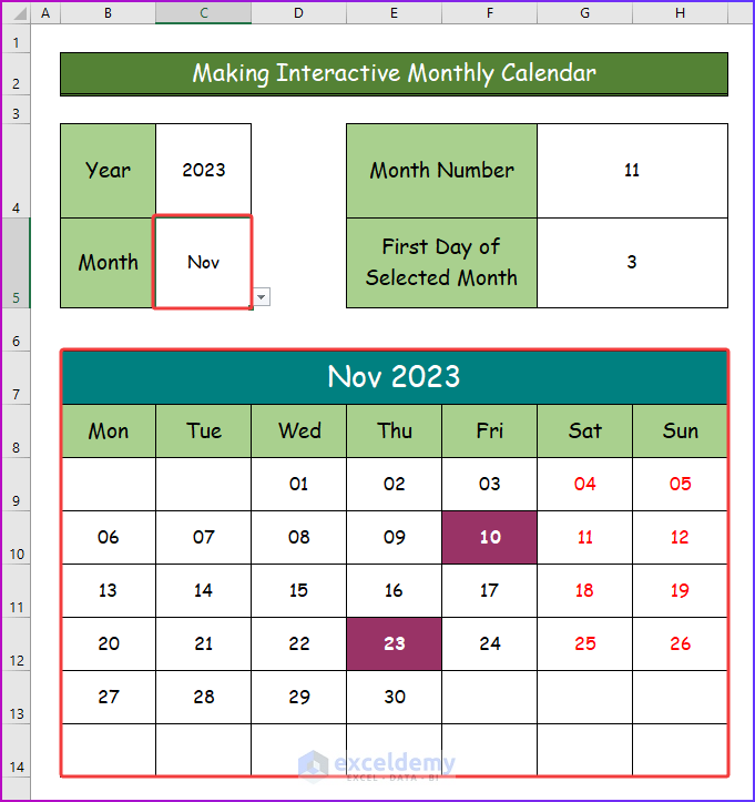
• The monthly calendar is ready as shown in the image below.

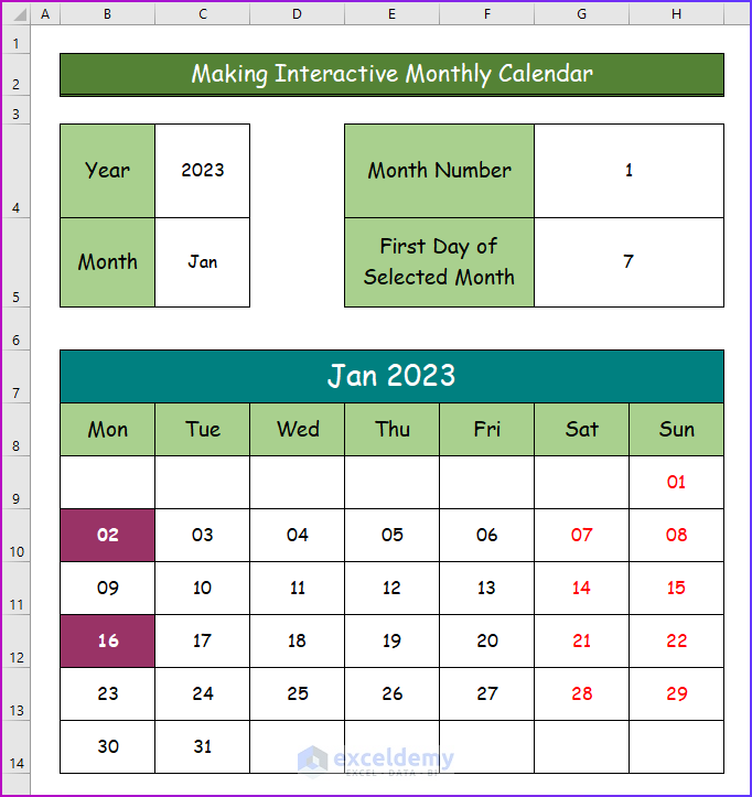
Step 31:

• Change the value of cell C5 to see the calendar for other months.

Read More: How to Make a Calendar in Excel Without Template

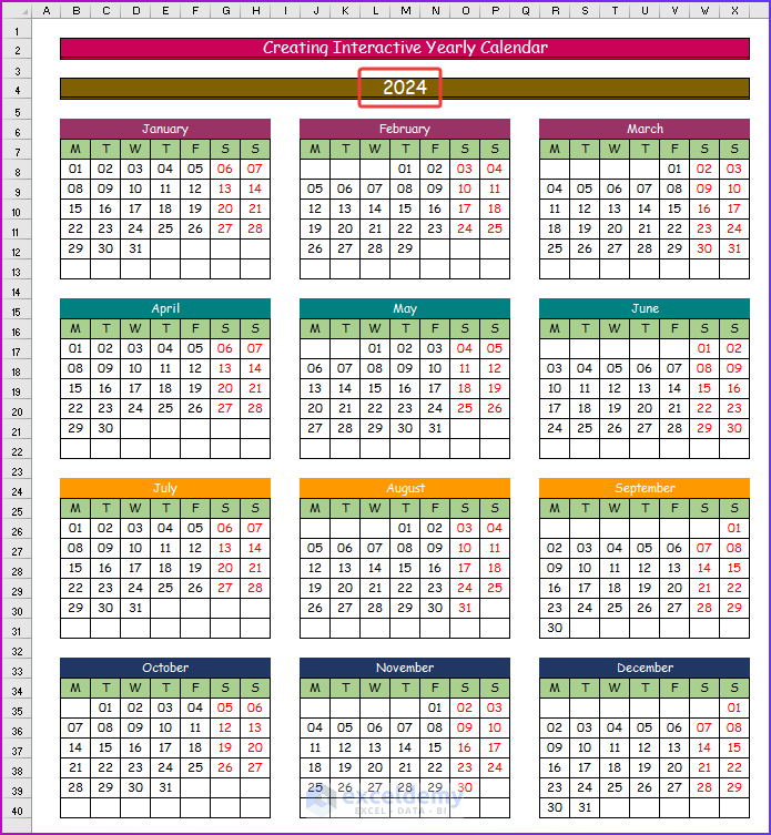
Method 2 – Creating Interactive Yearly Calendar in Excel

Step 1:

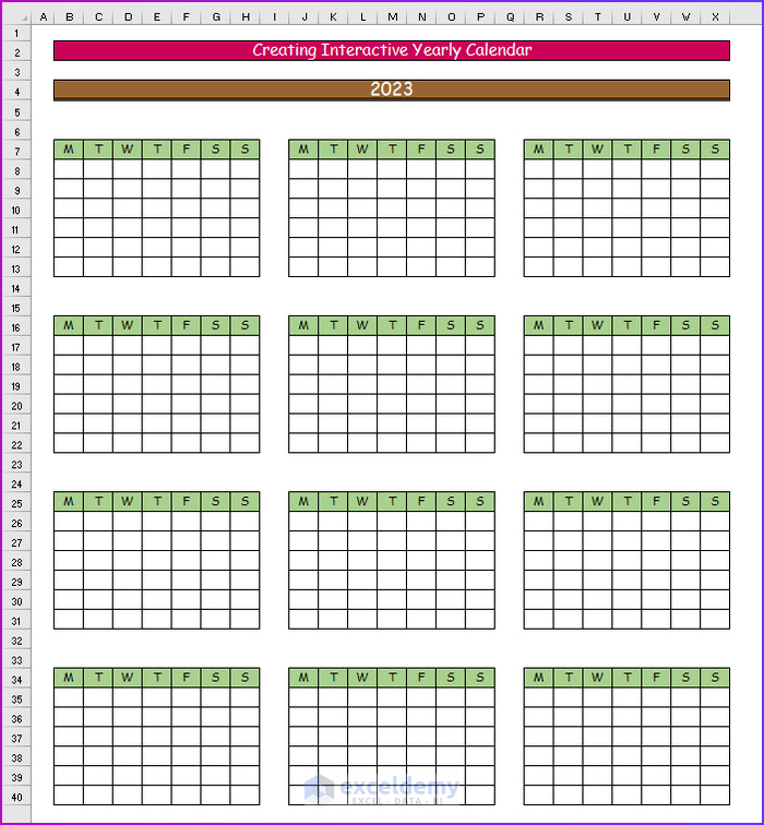
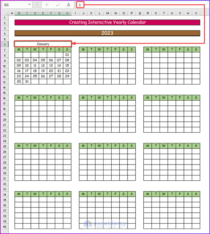
• Make twelve 7×7 tables as shown in the image below.
• Enter the days of the week starting from Monday in the tables.

Step 2:

• Enter 1 in cell B6 which is positioned just above the first table.

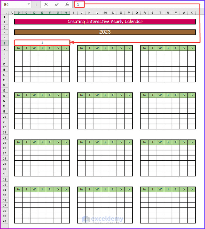
Step 3:

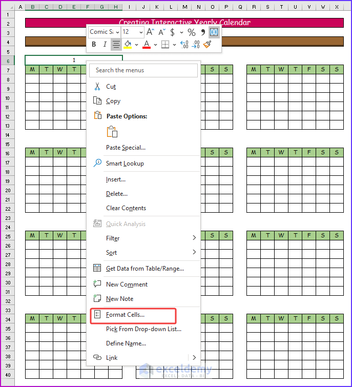
• Press Enter and right-click on cell B6.
• From the context, select Format Cells.

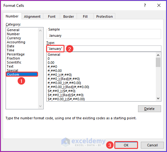
Step 4:

• The Format Cells dialog box will open.
• Go to the Custom tab and under the Type header, enter January.
• Press OK.

Step 5:

• Press OK.

Step 6:

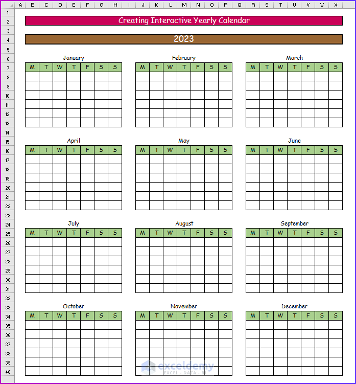
• Name all the tables as the twelve months in the form of numbers from 1-12.

Step 7:

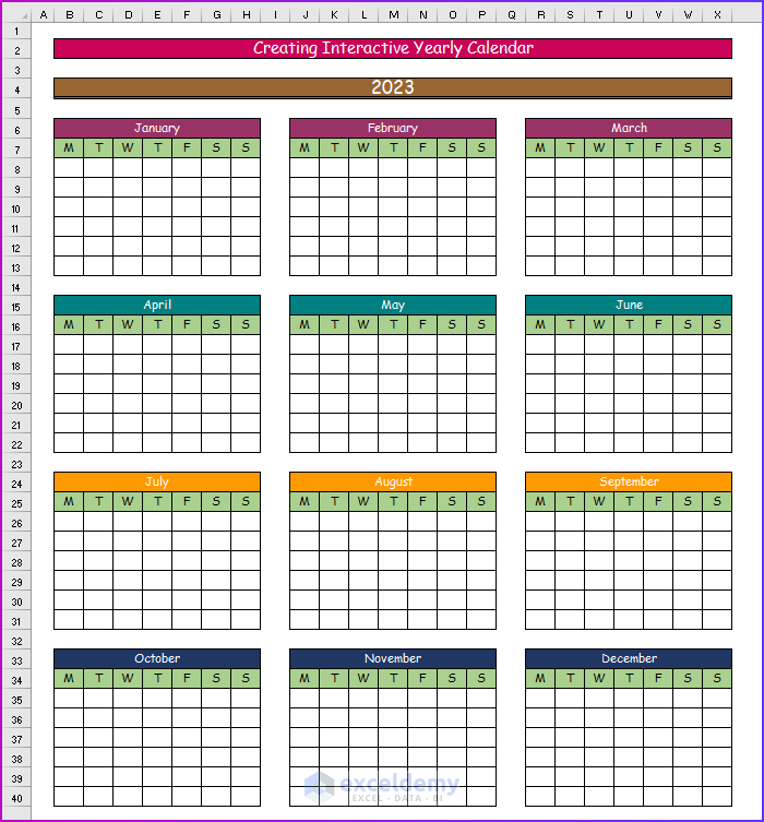
• Color the header of the table.

Step 8:

• To create the dates for the first month, enter the following formula in cell B8.

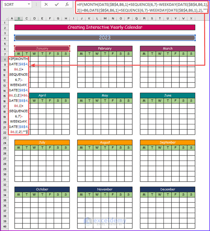
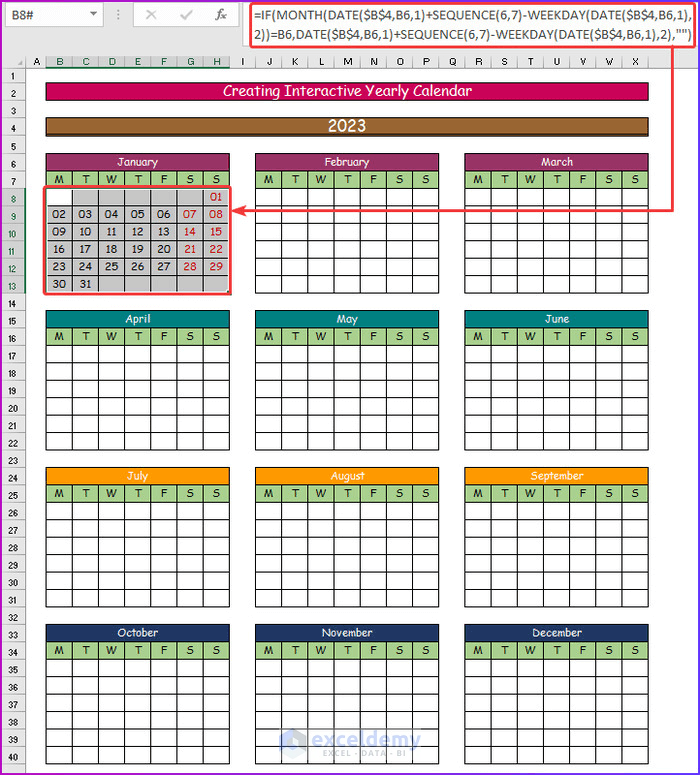
Step 9:

• Press Enter to get the dates for January 2023 in a correct sequence.
• Change the font color to red for the weekends.

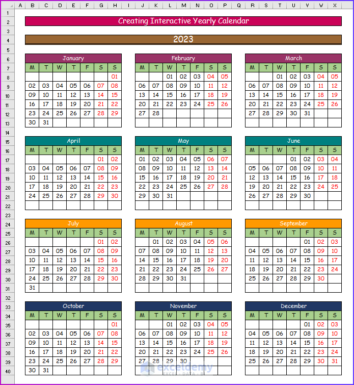
Step 10:

• Enter the formula for all the months to get the respective dates as shown in the image below.

Step 11:

• Select cell range B8:H13, to highlight the holidays for the first month of the year.

Step 12:

• Go to the Home tab and select Conditional Formatting.
• Choose the New Rule command from the dropdown.

Step 13:

• Edit the Edit Formatting Rule box as shown in the monthly calendar section. Use the formula below.

• Press OK.

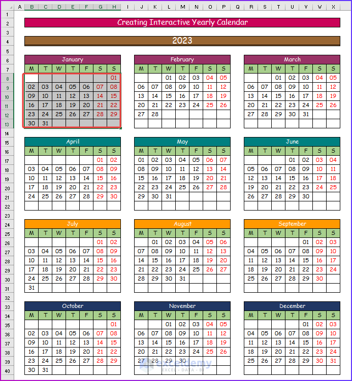
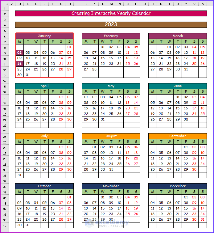
Step 14:

• All the holidays for the month of January are highlighted as shown in the image below.

Step 15:

• Use Conditional Formatting for the other eleven months to highlight their holidays.

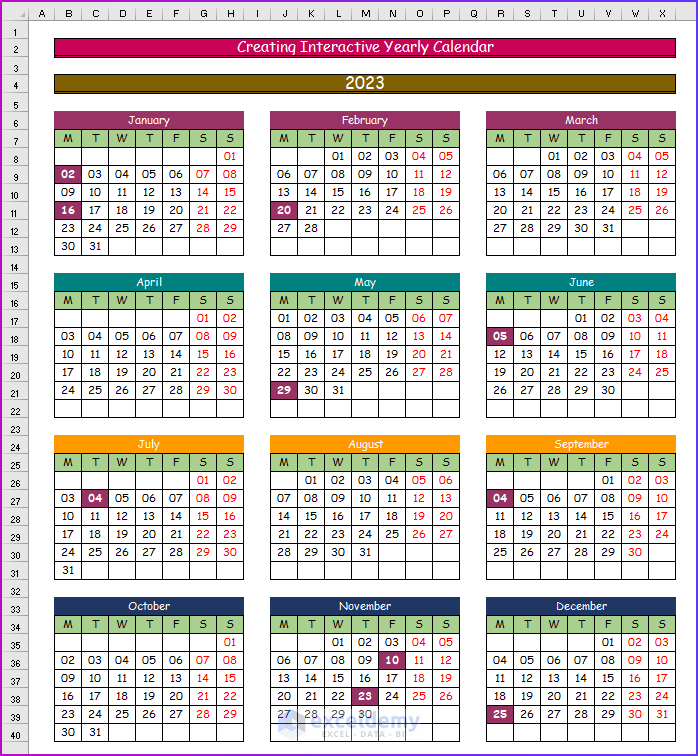
Step 16:

• Change the year value in cell B4 to see the year’s calendar.

Read More: How to Create a Yearly Calendar in Excel

Download Practice Workbook

Related Articles

• How to Create a Weekly Calendar in Excel
• How to Make a Blank Calendar in Excel