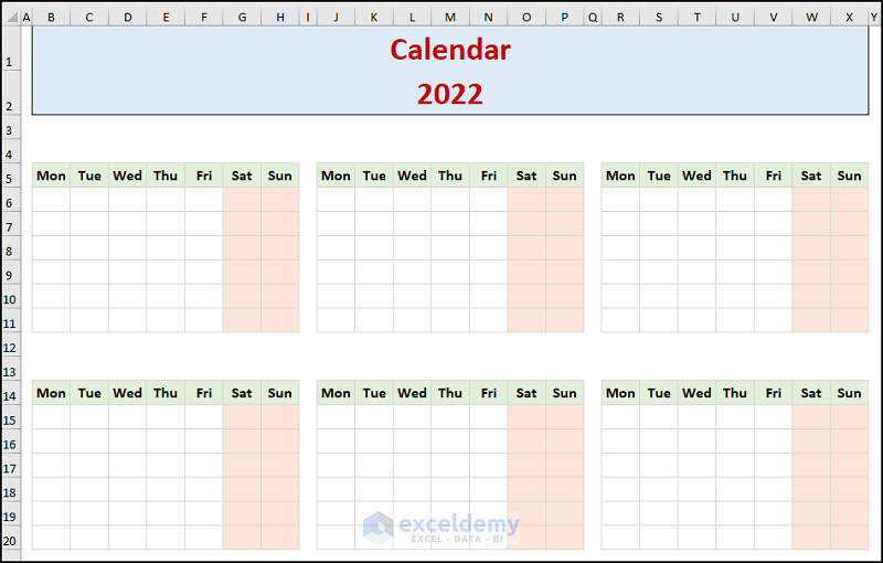
Method 1 – Create a Primary Outline
- Create an outline of the calendar by dividing the Months across 3 columns and 4 rows.
- Enter the 7 days in a Week and highlight the Weekends; Saturdays and Sundays.
Method 2- Enter Month Names
- Go to the B4 cell >> type in the number 1 >> hit the CTRL + 1 keys on your keyboard.
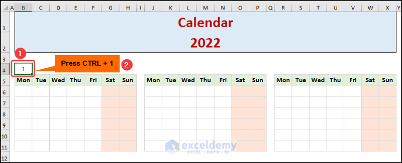
This opens the Format Cells dialog box.
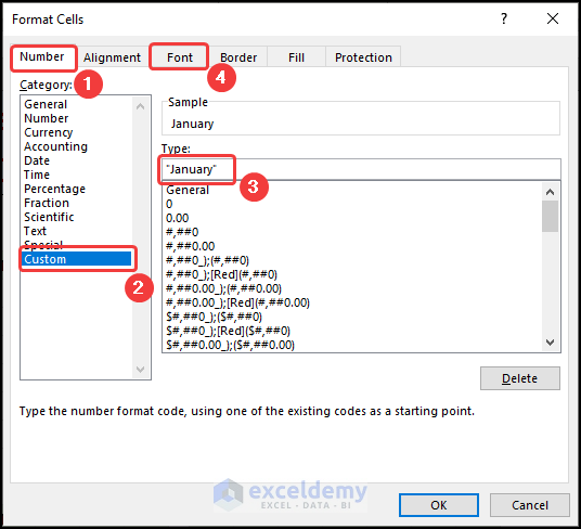
- Move to the Number tab >> choose Custom >> in the Type field, enter “January” (within inverted commas) >> jump to the Font tab.
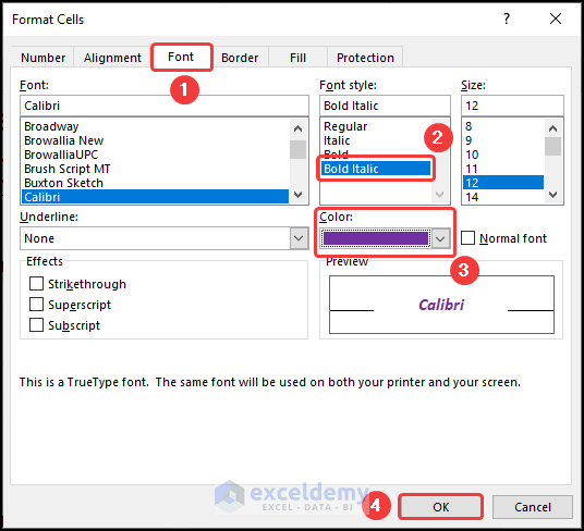
- Choose the Bold-Italic Font style >> select a Color, we chose purple >> hit OK.
- Select the B4:H4 range of cells >> press CTRL + 1 keys to navigate to the Format Cells window.
- Pproceed to the Alignment tab >> in the Horizontal section, choose Center Across Selection >> press OK.
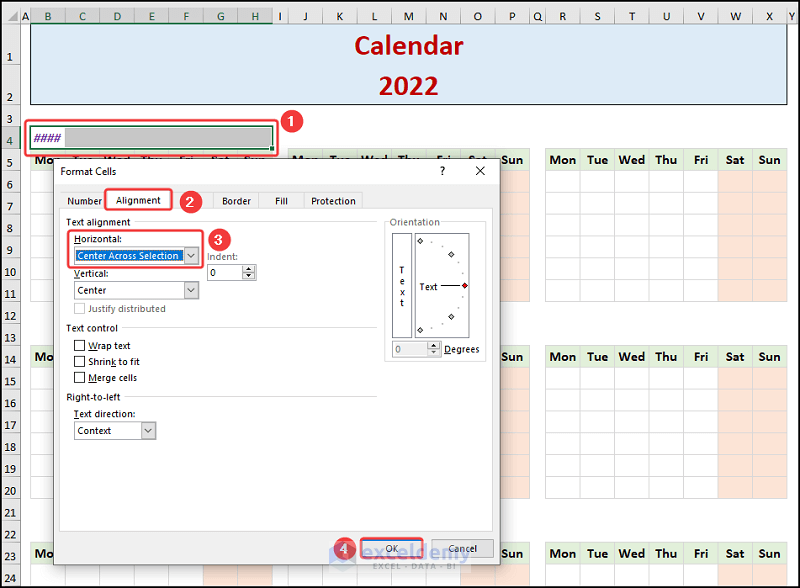
This should display the month name January, as shown in the image below.
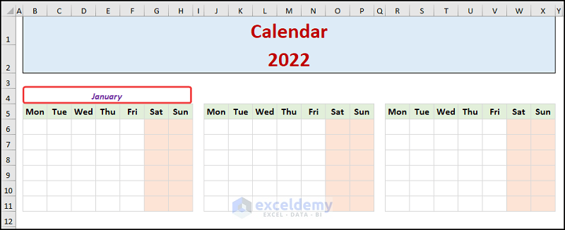
- Repeat the same procedure for the other months; your output should look like the following picture.
Method 3 – Utilize Excel Functions to Make Dynamic Calendar
- Move to the B6 cell and enter the formula given below.
=IF(MONTH(DATE($B$2,$B$4,1)+SEQUENCE(6,7)-WEEKDAY(DATE($B$2,$B$4,1),2))=$B$4,DATE($B$2,$B$4,1)+SEQUENCE(6,7)-WEEKDAY(DATE($B$2,$B$4,1),2),"")
The B2 and B4 cells refer to the Year 2022 and the Month of January, respectively.
Note: The SEQUENCE function is available on Excel 365, Excel 2021, and Excel for the web, so please make sure to have the compatible version.
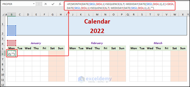
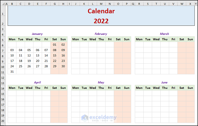
- Press the ENTER key, and the formula will populate all the days for the Month of January.
Note: Make sure to change the Date format to only dd in the Format Cells window by pressing the CTRL + 1 keys on your keyboard.
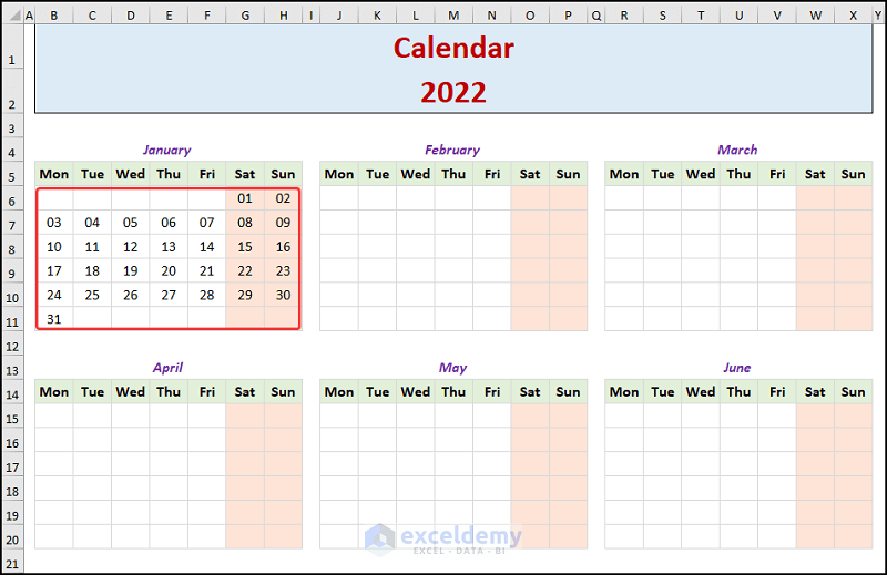
The result should look like the image below.
Method 4 – Indicate Holidays in the Calendar
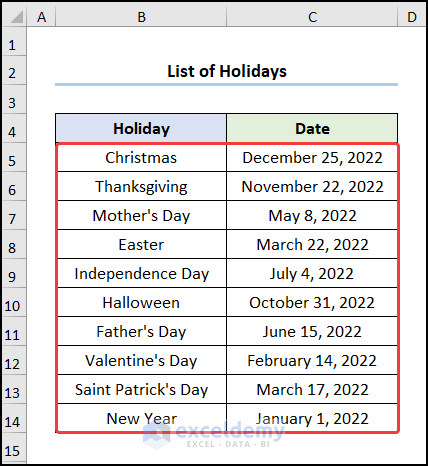
- Make a List of the Holidays in a new sheet as shown below.
- Select the B6:H11 cells >> go to the Conditional Formatting drop-down >> choose New Rule.
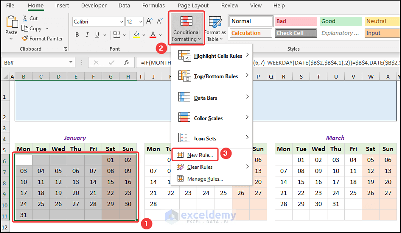
The New Formatting Rule wizard pops up.
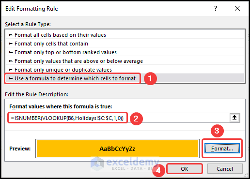
- Choose the Use a formula to determine which cells to format option.
- In the Rule Description enter the following formula.
=ISNUMBER(VLOOKUP(B6,Holidays!$C:$C,1,0))
The B6 cell points to the Monday in the Month of January while the Holidays!$C:$C represents the Dates in the Holidays sheet.
Formula Breakdown:
- VLOOKUP(B6,Holidays!$C:$C,1,0)) → the VLOOKUP function looks for a value in the left-most column of a table, and then returns a value in the same row from a column you specify. B6 ( lookup_value argument) is mapped from the Holidays!$C:$C (table_array argument) array. 1 (col_index_num argument) represents the column number of the lookup value. 0 (range_lookup argument) refers to the Exact match of the lookup value.
- Output → #N/A
- ISNUMBER(VLOOKUP(B6,Holidays!$C:$C,1,0)) → becomes
- ISNUMBER(#N/A) → the ISNUMBER function checks whether a value is a number and returns TRUE or FALSE. #N/A is the value argument, and since it is not a number, the function returns FALSE.
- Output → FALSE
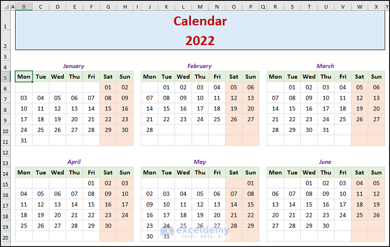
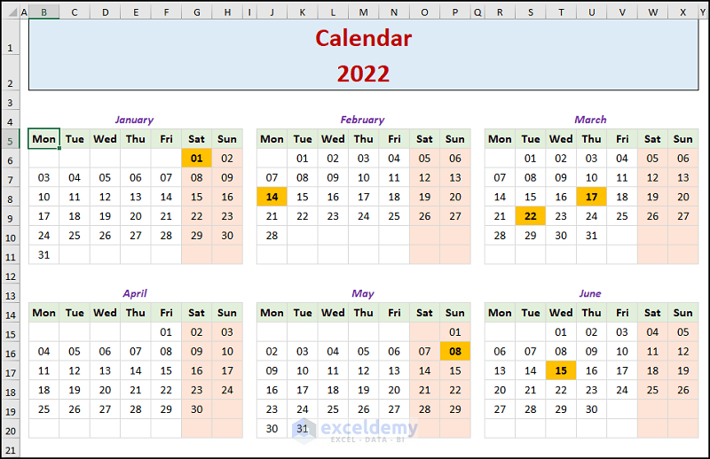
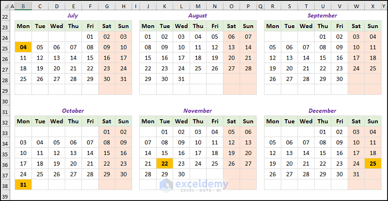
This should highlight the holiday on January 1st in bright orange color.
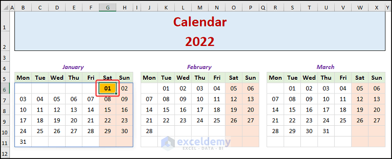
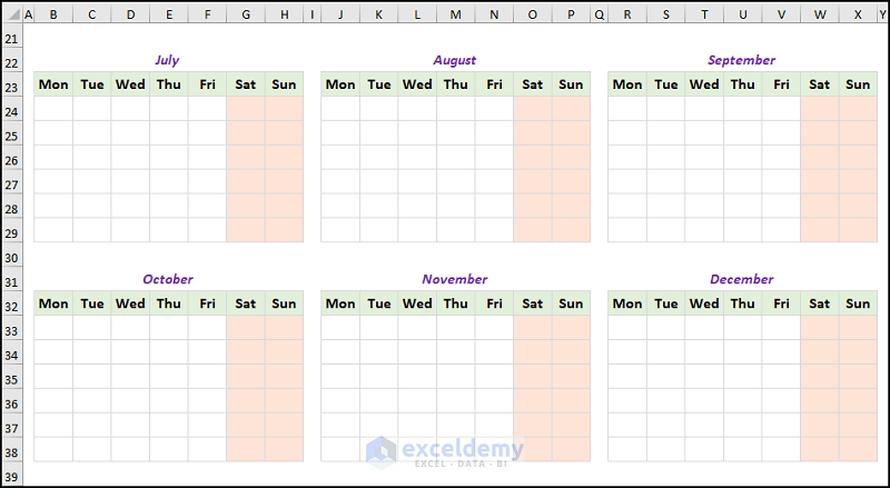
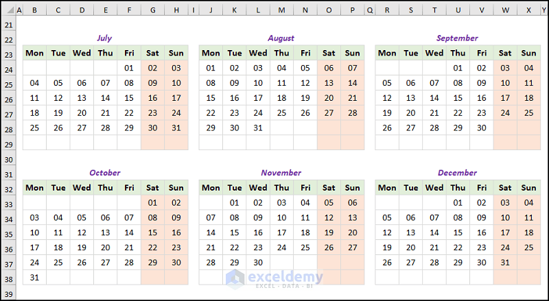
Repeat the same process for the other months and your output should look like the screenshots shown below.
How to Create a Monthly Calendar
Steps:
- Navigate to the Developer tab >> click Visual Basic.
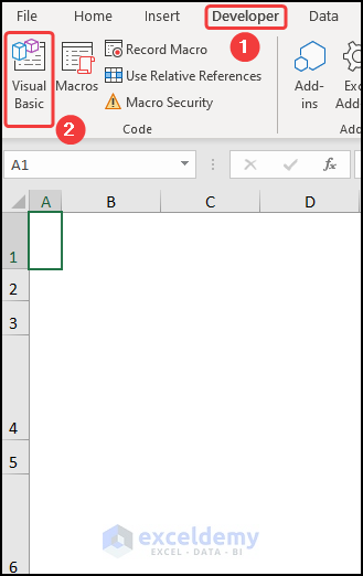
This opens the Visual Basic Editor in a new window.
- Go to the Insert tab >> select Module.
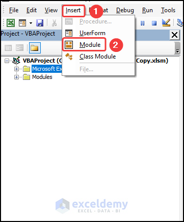
You can copy the code from here and paste it into the window as shown below.
Sub CalendarMaker()
'This code was taken from extendoffice.com
       ActiveSheet.Protect DrawingObjects:=False, Contents:=False, _
          Scenarios:=False
       Application.ScreenUpdating = False
       On Error GoTo MyErrorTrap

       Range("a1:g14").Clear
       MyInput = InputBox("Type in Month and year for Calendar ")
       If MyInput = "" Then Exit Sub
       StartDay = DateValue(MyInput)
       If Day(StartDay) <> 1 Then
           StartDay = DateValue(Month(StartDay) & "/1/" & _
               Year(StartDay))
       End If

       Range("a1").NumberFormat = "mmmm yyyy"
       With Range("a1:g1")
           .HorizontalAlignment = xlCenterAcrossSelection
           .VerticalAlignment = xlCenter
           .Font.Size = 18
           .Font.Bold = True
           .RowHeight = 35
       End With

       With Range("a2:g2")
           .ColumnWidth = 11
           .VerticalAlignment = xlCenter
           .HorizontalAlignment = xlCenter
           .VerticalAlignment = xlCenter
           .Orientation = xlHorizontal
           .Font.Size = 12
           .Font.Bold = True
           .RowHeight = 20
       End With

       Range("a2") = "Sunday"
       Range("b2") = "Monday"
       Range("c2") = "Tuesday"
       Range("d2") = "Wednesday"
       Range("e2") = "Thursday"
       Range("f2") = "Friday"
       Range("g2") = "Saturday"

       With Range("a3:g8")
           .HorizontalAlignment = xlRight
           .VerticalAlignment = xlTop
           .Font.Size = 18
           .Font.Bold = True
           .RowHeight = 21
       End With

       Range("a1").Value = Application.Text(MyInput, "mmmm yyyy")
       DayofWeek = Weekday(StartDay)
       CurYear = Year(StartDay)
       CurMonth = Month(StartDay)
       FinalDay = DateSerial(CurYear, CurMonth + 1, 1)
       Select Case DayofWeek
           Case 1
               Range("a3").Value = 1
           Case 2
               Range("b3").Value = 1
           Case 3
               Range("c3").Value = 1
           Case 4
               Range("d3").Value = 1
           Case 5
               Range("e3").Value = 1
           Case 6
               Range("f3").Value = 1
           Case 7
               Range("g3").Value = 1
       End Select

       For Each cell In Range("a3:g8")
           RowCell = cell.Row
           ColCell = cell.Column
           If cell.Column = 1 And cell.Row = 3 Then
           ElseIf cell.Column <> 1 Then
               If cell.Offset(0, -1).Value >= 1 Then
                   cell.Value = cell.Offset(0, -1).Value + 1

                   If cell.Value > (FinalDay - StartDay) Then
                       cell.Value = ""
                       Exit For
                   End If
               End If

           ElseIf cell.Row > 3 And cell.Column = 1 Then
               cell.Value = cell.Offset(-1, 6).Value + 1
               If cell.Value > (FinalDay - StartDay) Then
                   cell.Value = ""
                   Exit For
               End If
           End If
       Next

       For x = 0 To 5
           Range("A4").Offset(x * 2, 0).EntireRow.Insert
           With Range("A4:G4").Offset(x * 2, 0)
               .RowHeight = 65
               .HorizontalAlignment = xlCenter
               .VerticalAlignment = xlTop
               .WrapText = True
               .Font.Size = 10
               .Font.Bold = False
               .Locked = False
           End With

           With Range("A3").Offset(x * 2, 0).Resize(2, _
           7).Borders(xlLeft)
               .Weight = xlThick
               .ColorIndex = xlAutomatic
           End With

           With Range("A3").Offset(x * 2, 0).Resize(2, _
           7).Borders(xlRight)
               .Weight = xlThick
               .ColorIndex = xlAutomatic
           End With
           Range("A3").Offset(x * 2, 0).Resize(2, 7).BorderAround _
              Weight:=xlThick, ColorIndex:=xlAutomatic
       Next
       If Range("A13").Value = "" Then Range("A13").Offset(0, 0) _
          .Resize(2, 8).EntireRow.Delete

       ActiveWindow.DisplayGridlines = False
       ActiveSheet.Protect DrawingObjects:=True, Contents:=True, _
          Scenarios:=True

       ActiveWindow.WindowState = xlMaximized
       ActiveWindow.ScrollRow = 1

       Application.ScreenUpdating = True
       Exit Sub

MyErrorTrap:
       MsgBox "You may not have entered your Month and Year correctly." _
           & Chr(13) & "Spell the Month correctly" _
           & " (or use 3 letter abbreviation)" _
           & Chr(13) & "and 4 digits for the Year"
       MyInput = InputBox("Type in Month and year for Calendar")
       If MyInput = "" Then Exit Sub
       Resume
   End Sub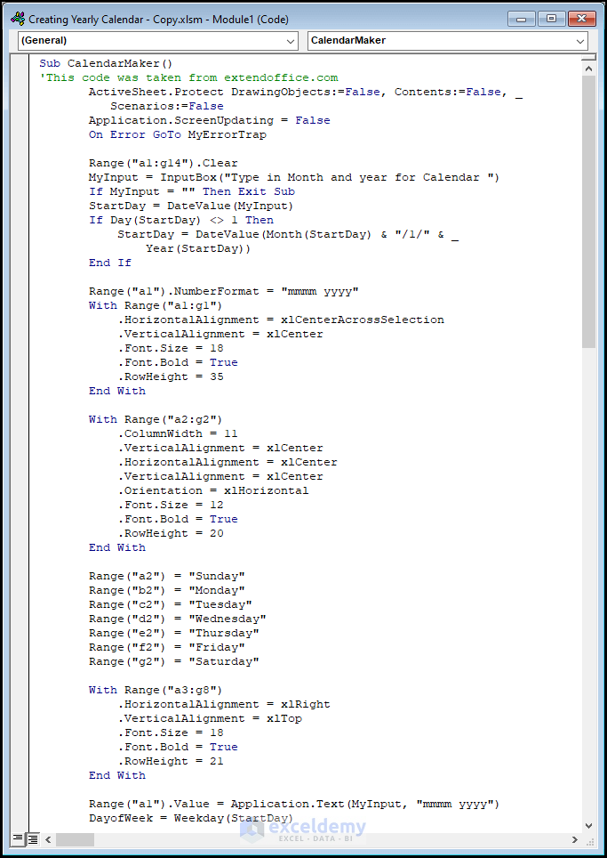
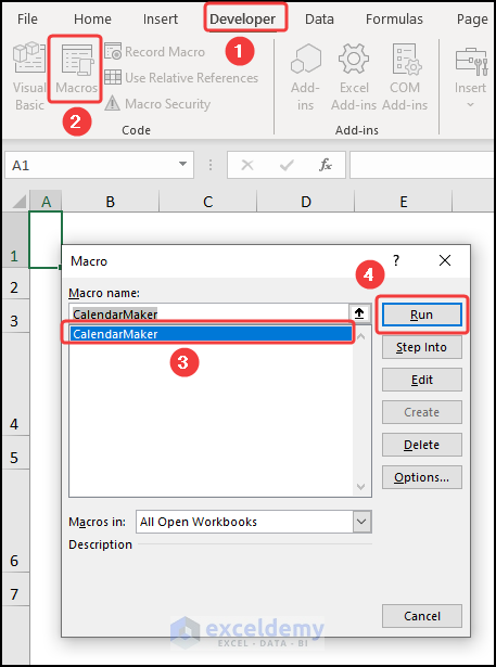
- Close the VBA window >> click Macros.
This opens the Macros dialog box.
- Select the CalendarMaker macro >> hit Run.
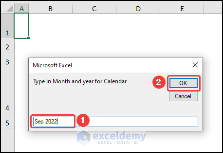
This opens an Input box >> enter the Month Name and Year as shown below.
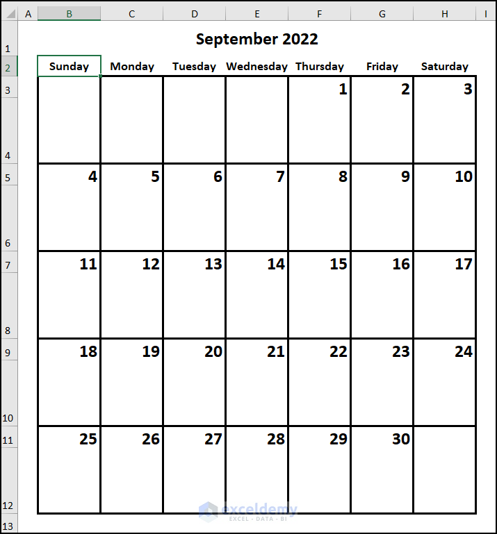
The results should look like the picture below.
Download Practice Workbook
You can download the practice workbook from the link below.
Related Article
- How to Make a Calendar in Excel Without Template
- How to Create a Weekly Calendar in Excel
- How to Make an Interactive Calendar in Excel
- How to Make a Blank Calendar in Excel
Get FREE Advanced Excel Exercises with Solutions!

