How to Forecast Sales Using Historical Data in Excel (6 Methods)

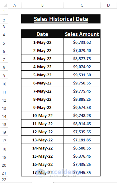
Suppose we have the Sales Amount for the first couple of dates in a month and we want to forecast the sales amount for the rest of the days in the month.

In this article, we demonstrate multiple features, FORECAST, TREND, and GROWTH functions as well as the manual method to forecast sales using historical data in Excel.

What Is Forecasting?

Forecasting is a method to generate a correlation between amount/quantity and trends depending on the available historical data. Forecasting is used to understand market trends and enable taking rational steps to accommodate the budget or requirements.

⧭ Forecasting is just a method to assume future events, not an exact prediction.

How to Forecast Sales Using Historical Data in Excel: 6 Easy Ways

There are several methods to find forecast data in Excel, each with its own shortcomings. You’ll have to determine which of the below methods best suits your objectives in each case.

Method 1 – Using Forecast Sheet Feature

Steps:

• Highlight the available historical data.
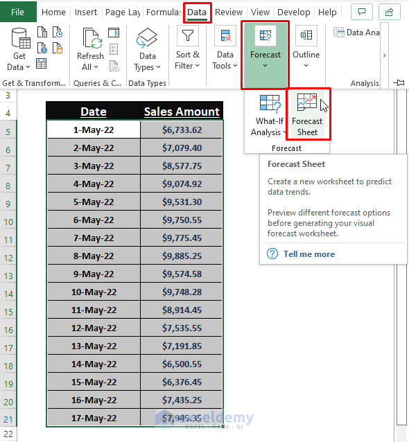
• Go to the Data tab.
• Click on Forecast Sheet (in the Forecast section).

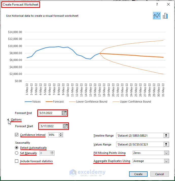
The Create Forecast Worksheet window opens.

• Provide necessary entries in the dialog boxes as depicted.
• Click on Create.

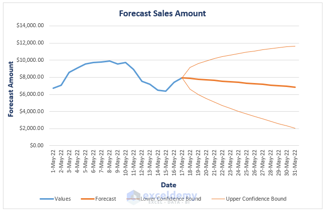
A new Worksheet with forecast Lower and Upper Bound values is inserted.

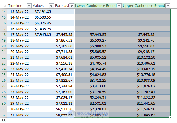
A Trend Chart depicting the forecasted Lower and Upper Bound along with the forecast values mimicking the historical data is also inserted.

Read More: How to Forecast in Excel Based on Historical Data

Method 2 – Using Moving Average

Moving Average property is found in multiple features of Excel. A typical moving average value is the average value of a dynamic handful (here it is 7) of entries. The Moving Average tool in the Data Analysis feature or the Trendline options’ Moving Average can forecast sales or anything using historical data.

2.1 – Typical Moving Average Forecast

Steps:

• In cell F6, use the AVERAGE function to find the average value of the first 7 entries (cells C5:C11) for the first forecast value (18-May):

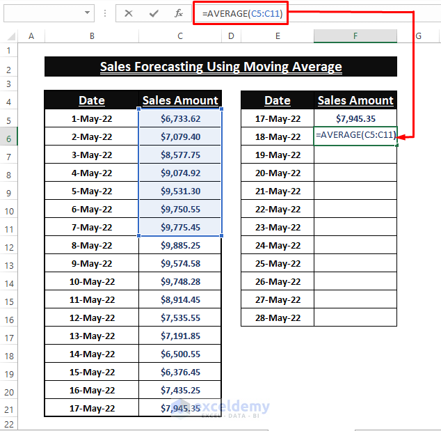
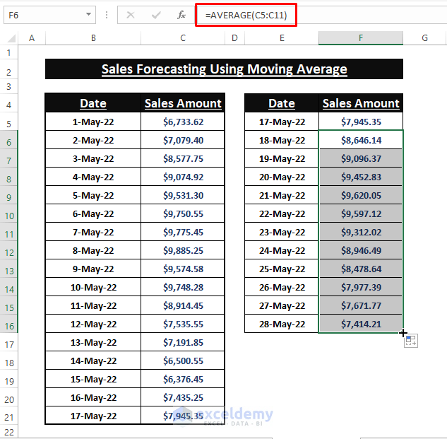
• Press ENTER and use the Fill Handle to display the forecasted values for the rest of the month.

2.2 – Data Analysis Moving Average

Steps:

• Go to the Data tab.
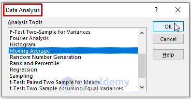
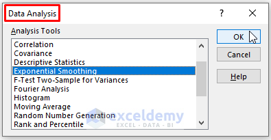
• Click on the Data Analysis feature in the Data Analysis section.
• Find and choose the Moving Average option within the Data Analysis tools.
• Click OK.

2.3 – Trendline Options

We can insert a Moving Average Trendline in the Line Chart depiction of the historical data. To do so, first insert a Line Chart of the available historical data.

Steps:

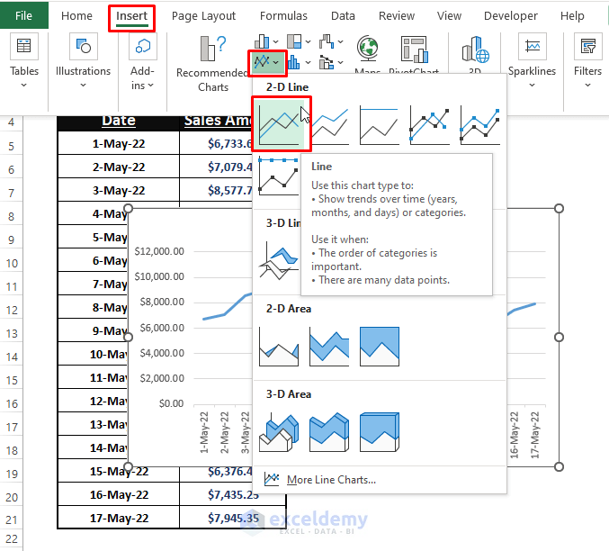
• Go to the Insert tab.
• Select Line (from the Charts section).

Excel automatically takes the existing data and inserts a Line Chart.

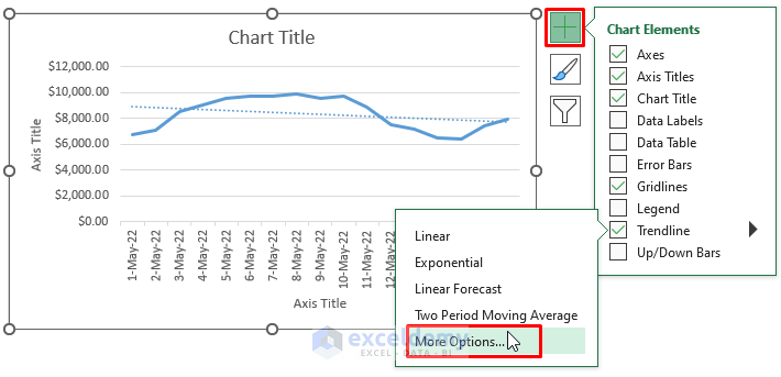
• Click on the Plus icon beside the Chart.
• Tick the Trendline option and click on the Arrow.
• Select More Options.

The Format Trendline window appears.

• Click on the Moving Average from the Format Trendline Options.

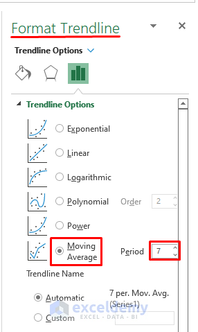
• Format the Line Chart as you desire.

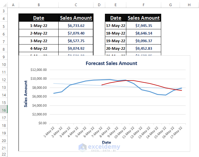
The forecasted values will be depicted as a Line (here it’s the red line) in the Chart.

Read More: How to Forecast Sales in Excel

Method 3 – Using FORECAST Function Variants

There are multiple variants of the FORECAST function, including FORECAST, FORECAST.LINEAR, and FORECAST.ETS.

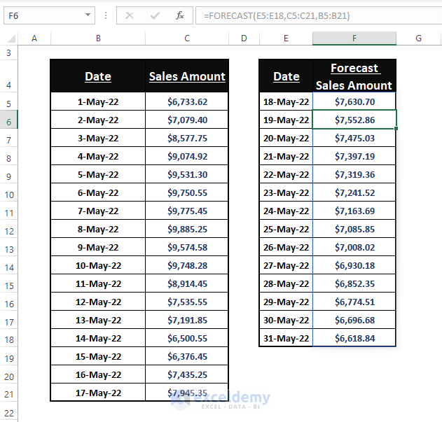
3.1 – Using FORECAST Function

The FORECAST function returns the linear trends maintaining the historical data. The syntax of the function is:

Steps:

• Paste the below formula in the desired cells:

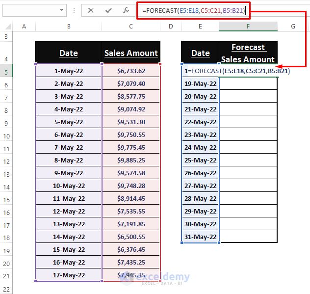
• Press CTRL+SHIFT+ENTER to display the forecasted values.

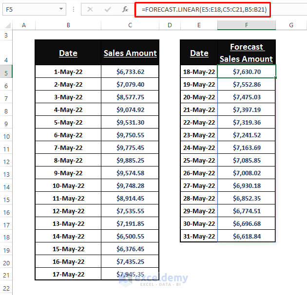
3.2 – Using FORECAST.LINEAR Function

Alternatively, the FORECAST.LINEAR function returns the future values mimicking the historical data trend. The syntax of the function is:

Steps:

• Use the below formula in any cell then hit CTRL+SHIFT+ENTER.

The forecasted data is returned instantly.

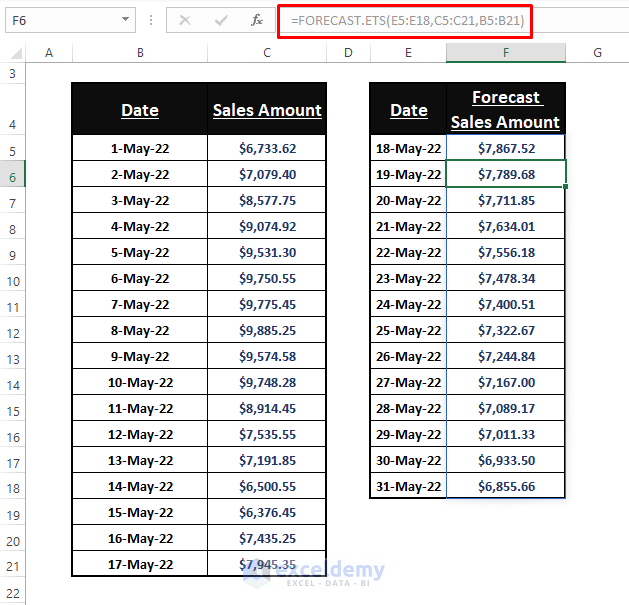
3.3 – Using FORECAST.ETS Function

To allow for seasonality trends in forecasted data, it’s preferable to use the FORCAST.ETS function. The syntax of the FORECAST.ETS function is:

Steps:

• Enter the following formula in any cell then press CTRL+SHIFT+ENTER to apply the formula:

The formula returns the forecasted data considering the seasonality in historical data trends.

• As an alternative to the FORECAST.ETS function, there is an Exponential Smoothing tool in the Data Analysis feature.

Read More: How to Forecast Sales Growth Rate in Excel

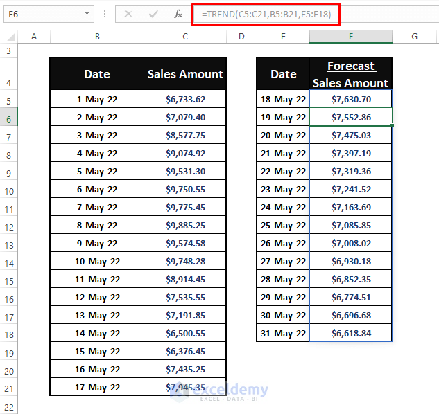
Method 4 – Using TREND Function

The TREND function fits the forecast data to the linear trend of the historical data. The function’s outcomes are linear trend values that sit on a straight line. The syntax of the function is:

Steps:

• Enter the following formula in any cell:

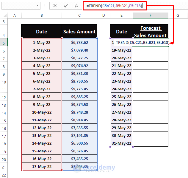
• Press CTRL+SHIFT+ENTER to display the outcomes.

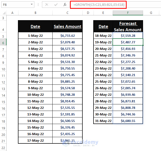
Method 5 – Using GROWTH Function

Exponential growth is predicted by the GROWTH function. The syntax of the function is

Steps:

• Enter the following formula in any desired cell:

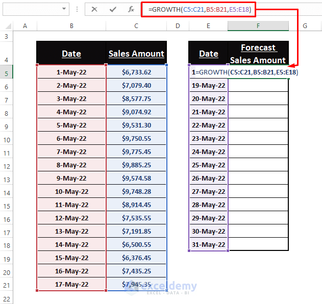
• As the function is an array function, use CTRL+SHIFT+ENTER to display the outcomes.

⧭ Use ENTER with array formulas if you are using the Excel 365 version.

Read More: How to Forecast Sales Using Regression Analysis in Excel

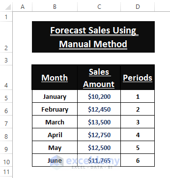
Method 6 – Using Manual Method

Suppose we have the first six months’ sales amounts as period data, and we want to use these sales data to forecast the next six months’ sales.

Steps:

• Use the below LINEST array formula to find the constant values of a linear equation. If the linear equation is Y= bX+c, the function results in both constant b and c.

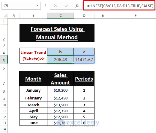
Now we find the trend values of monthly sales.

• Paste the below formula in cell E8:

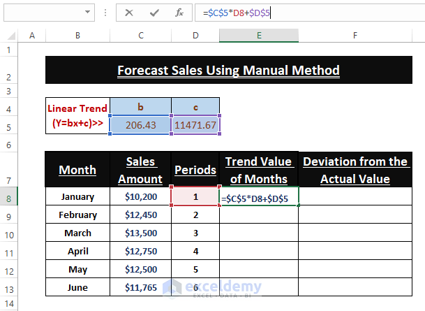
• Use the Fill Handle to populate the trend values.
• Find the deviation of the actual value from the trend by dividing Actual Value by the Trend value:

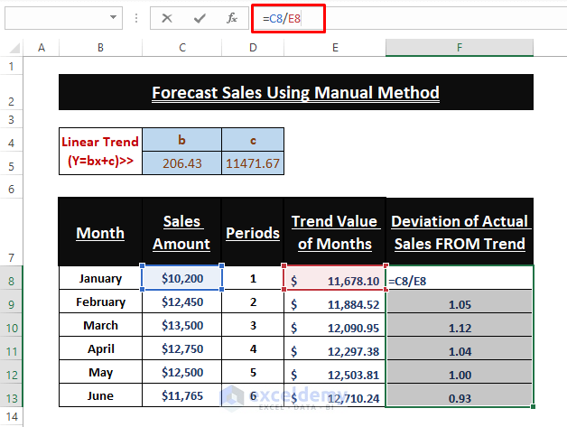
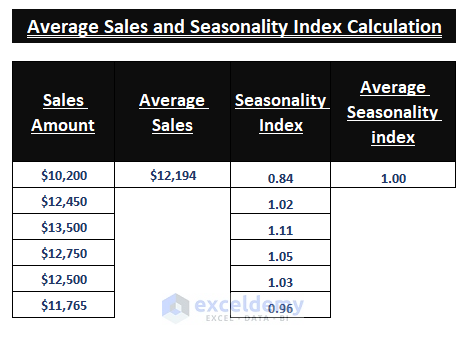
• Calculate the Average Sales (using the AVERAGE function), Seasonality Index (Sales Amount/Average Sales) and Average Seasonality Index (using the AVERAGE function).

• Find the trend value for the next 6 months using the below formula:

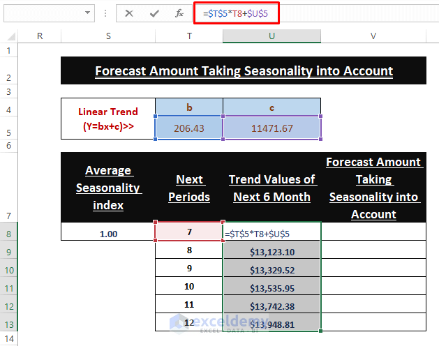
• Finally, multiply the seasonality index with trend values to find the forecast sales amount taking seasonality into account.

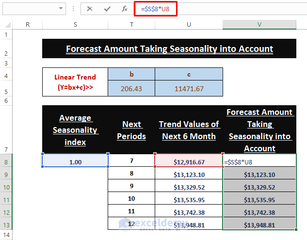
Read More: How to Do Budgeting and Forecasting in Excel

Download Excel Workbook

Related Articles

• How to Forecast Growth Rate in Excel
• How to Forecast Revenue in Excel
• How to Forecast Revenue Growth in Excel

<< Go Back to Excel for Finance | Learn Excel