The following image showcases a setup of a two-variable data table.
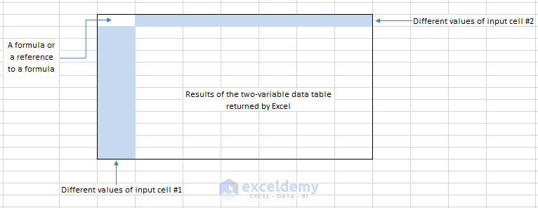
The setup of a two-variable data table.
Example 1 – Creating a Two Variable Data Table for a Direct Mail Profit Model
In this example, a company wants to make a direct-mail promotion to sell its product.
This data table model uses two input cells: the number of letters sent and the expected response rate. There are more items in the Parameters area.
This worksheet calculates the net profit of the direct-mail promotion.
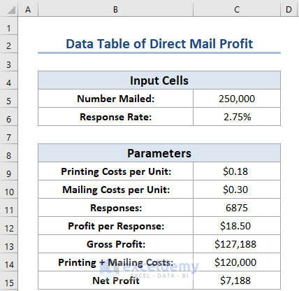
Parameters:
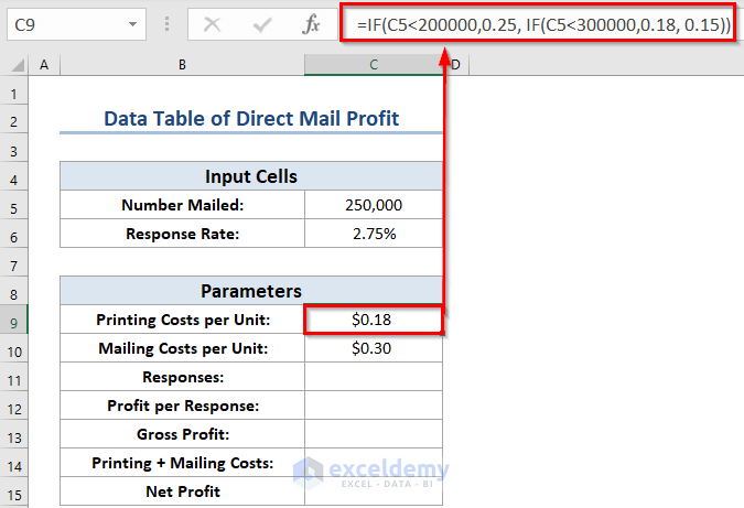
Printing Costs per Unit: the cost to print a letter. The unit cost varies with the quantity: $0.25 each for quantities less than 200,000; $0.18 each for quantities between 200,001 and 300,000; and $0.15 for more than 300,000.
- The following formula was used in C9.
=IF(C5<200000,0.25, IF(C5<300000,0.18, 0.15))- Mailing Costs per Unit: It is a fixed cost, $0.30 per letter mailed.
- Responses: The number of responses, is calculated from the response rate and the number mailed.
- The formula is the following:
=C5*C6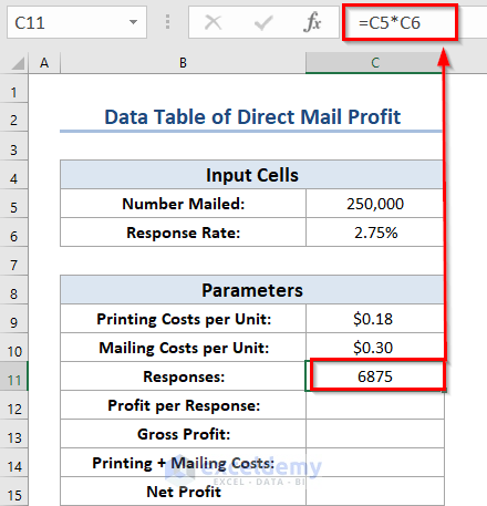
- Profit per Response: It is also a fixed value. The company knows that it will have an average profit of $18.50 per order.
- Gross Profit: The formula multiplies the profit-per-response by the number of responses:
=C11*C12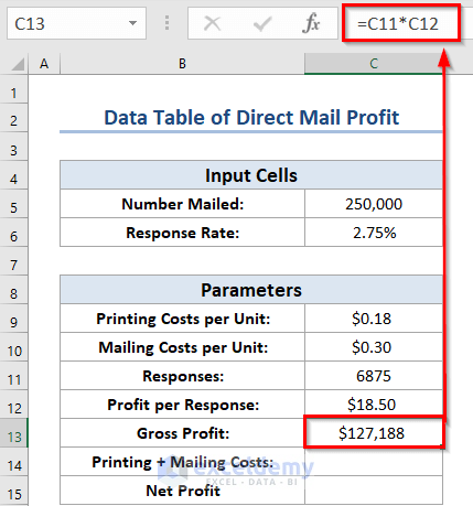
- Print + Mailing Costs: This formula calculates the total cost of the promotion:
=C5*(C9+C10)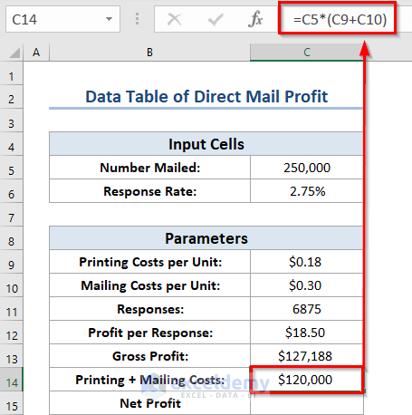
- Net Profit: This formula calculates the bottom line – the gross profit minus the printing and mailing costs.
- It was used in C15.
=C13-C14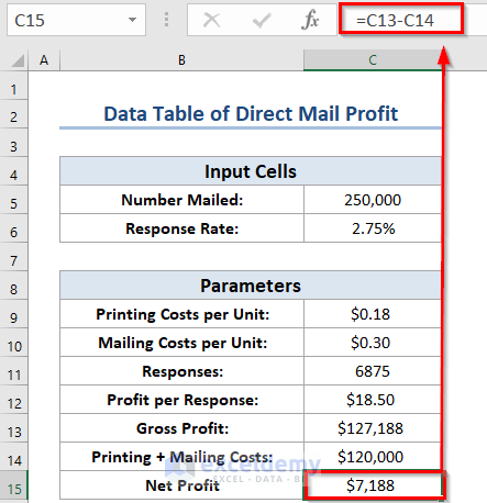
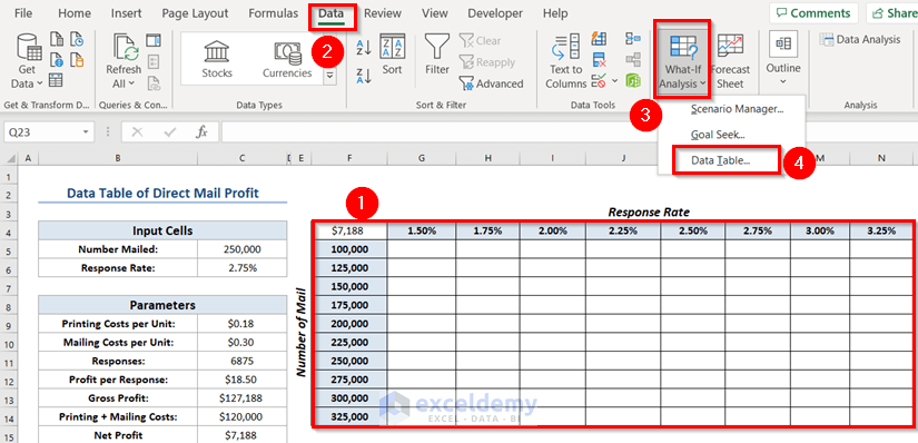
The image below shows the setup of a two-variable data table that summarizes the net profit with different combinations of mail numbers and response rates.
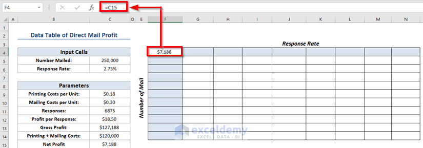
- Enter the Response Rate values in G4: N4.
- Enter the Number of Mail values in F5: F14.
- Select F4:N14.
- In the Data tab >> Go to the What-If Analysis command.
- Choose Data Table.
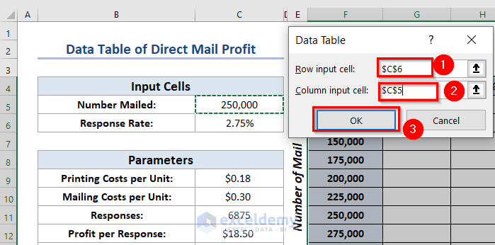
In the Data Table dialog box:
- Specify C6 as the Row input cell (Response Rate).
- Select C5 as the Column input cell (Number Mailed).
- Click OK.
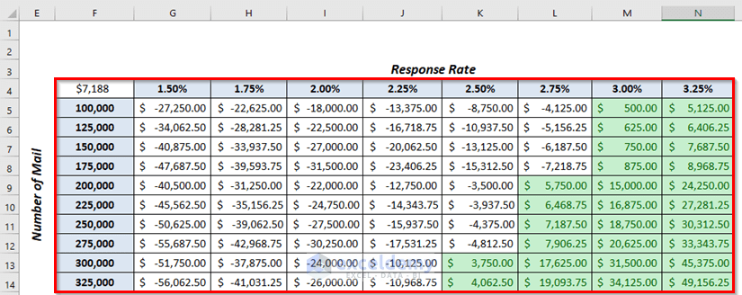
Excel fills the data table and returns the final result:
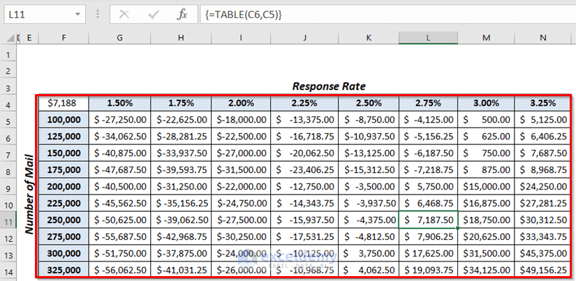
The data table is dynamic. You can change the formula in F4 to refer to another cell (Gross Profit) or enter different values in Response Rate and Number Mailed.
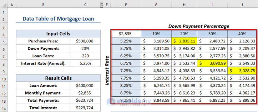
Example 2 – Creating a Two Variable Data Table of a Loan Payment
Calculate the Monthly Payment.
- Select C12 to display the Monthly Payment.
- Use the formula:
=PMT(C8/12,C7,-C11)- Press ENTER.
The Monthly Payment is displayed.
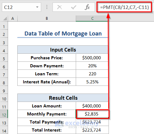
Formula Breakdown
the PMT function calculates the payment based on a loan with a constant interest rate and regular payment.
- C8 denotes the annual interest rate of 5.25%.
- C7 denotes the total payment period: 220 months.
- C11 denotes the present value: $400,000.
The following figure shows the setup of a two-variable data table that summarizes the monthly payment with different combinations of Interest Rate and Down Payment Percentage.
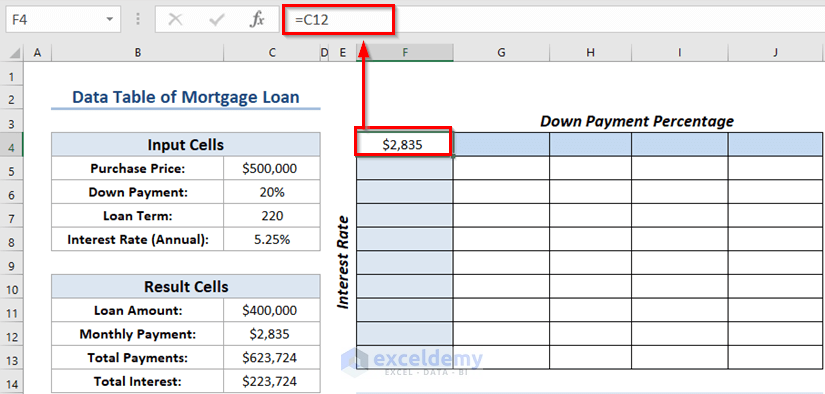
- Enter the Down Payment Percentage in G4: J4.
- Enter the Interest Rate in F5: F13.
- Select F4:J13.
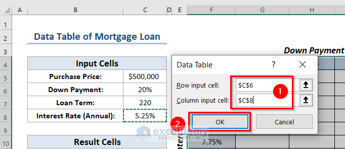
- In the Data tab >> Go to What-If Analysis.
- Choose Data Table.

In the Data Table dialog box:
- Specify C6 as the Row input cell (Down Payment).
- Select C8 as the Column input cell (Interest Rate).
- Click OK.
Excel fills the data table.
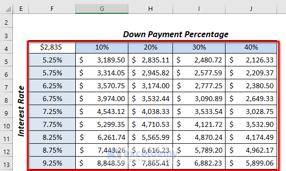
Cells containing the target monthly payment were highlighted
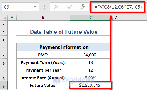
Example 3 – Creating a Two Variable Data Table of the Future Value
Calculate the Future Value.
- Select C12 to calculate the Future Value.
- Use the formula:
=FV(C8/12,C6*C7,-C5)- Press ENTER to see the result.
You will see the amount of the Future Value.
Formula Breakdown
- the FV function returns the Future Value of the periodic investment.
- C8 denotes the Annual Interest Rate.
- C6 denotes the total time period as Year.
- C5 denotes the monetary value that you are paying at present.
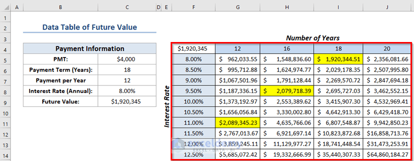
Create a two-variable data table that summarizes the Future Value with different combinations of Interest Rate and Number of Years.
This is the final data table.
Download Working File
Download the file from the link below:
Related Articles
- How to Create One Variable Data Table in Excel
- How to Create One Variable Data Table Using What-If Analysis
- How to Create Data Table with 3 Variables
- How to Create a 4-Variable Data Table in Excel
<< Go Back to Data Table in Excel | What-If Analysis in Excel | Learn Excel
Get FREE Advanced Excel Exercises with Solutions!

I Have been following your Data analysis articles such as how to create variable tables. I just downloaded the lessons because of the nature of my work as a journalist.
Now that I have started actually studying them, I found your method of teaching worth commending. They are just what you termed them, “step by step” and they are actually straight to the point, easy to follow, easy to understand.
I also want to thank the owner of trumpexcel.com/excel website who directed my attention to your web when I was studying his 100 excel questions series.
Your work is really commendable.
Thanks.
Uche Uche.
Thanks for your feedback, Uche Uche.
Feeling happy to know that you found the articles helpful.
Best regards
Kawser Ahmed