How to Create a Data Table with 3 Variables – 2 Examples

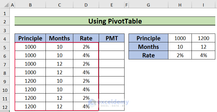
Example 1 – Using a PivotTable to Create a Data Table with 3 Variables

Use the PMT function.

Steps:

• Enter Principle, Months, and Rates in B5:D12.

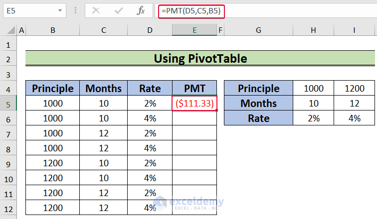
• Click E5 and enter the following formula.

• Press Enter.

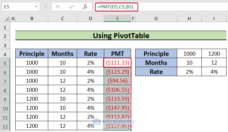
This is the output.

• Drag down the Fill Handle to autofill the formula.

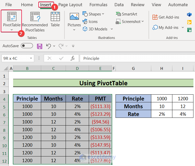
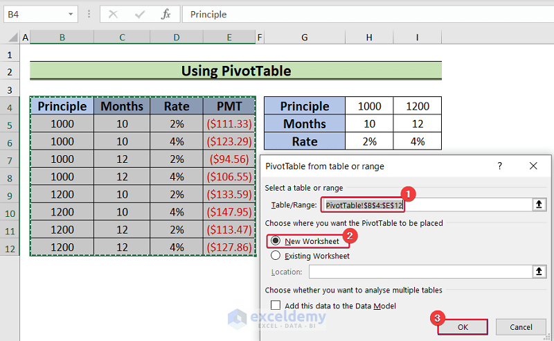
• Select B5:E12.
• Go to the Insert tab.
• Select PivotTable.

• Select B5:E12 in Table /Range.
• Select New Worksheet.
• Click OK.

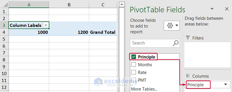
• In the new worksheet, drag Principle to Columns.

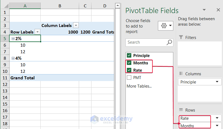
• Drag Months and Rate to Rows.

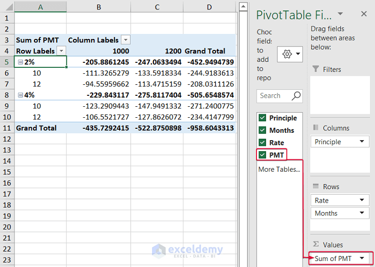
• Drag PMT to Values.

The pivot table is created.

• Click a cell in the pivot table.
• Go to the Design tab.
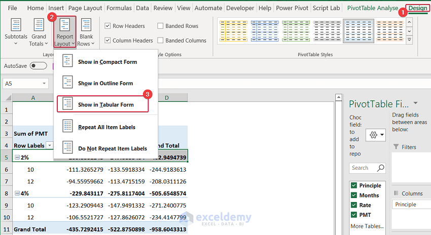
• Select Report Layout tab.
• Choose Show in Tabular Form.

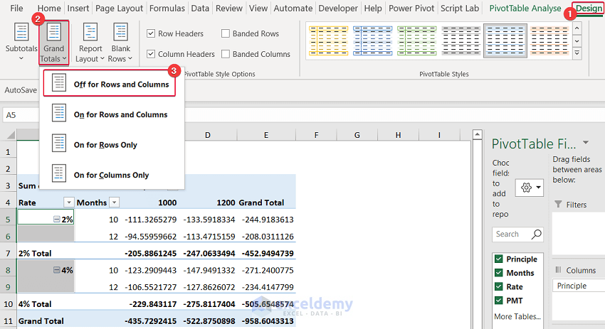
• Click a cell in the pivot table.
• Go to the Design tab.
• Select Off for Rows and Columns in Grand Totals.

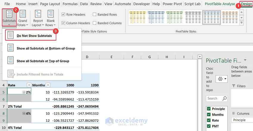
• Go to the Design tab.
• In Subtotal, select Do Not Show Subtotals.

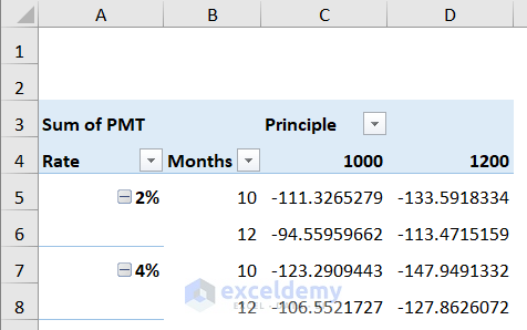
This is the output: a data table with 3 variables.

Read More: How to Create One Variable Data Table in Excel

 Example 2 – Using the Data Table Command

Use the SUMPRODUCT function.

Steps:

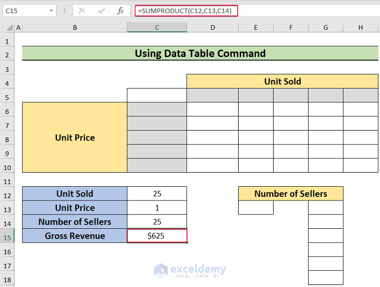
• Select C15 and enter the formula below.

• Press Enter.

This is the output.

• Click D5 and enter:

• Press Enter.

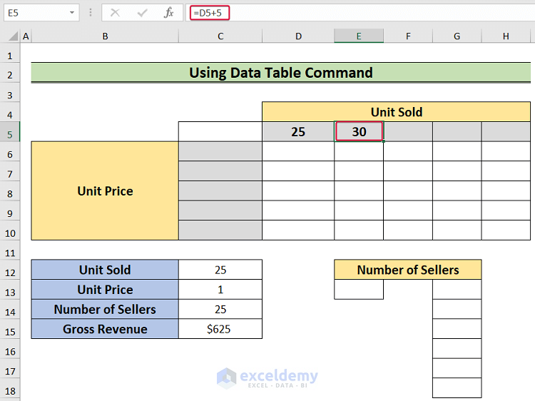
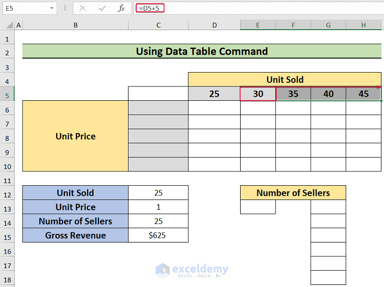
• Select E5 and enter the formula below.

• Press Enter.

• Drag down the Fill Handle to see the result in the rest of the cells.

• Choose C6 and enter the following formula.

• Press Enter.

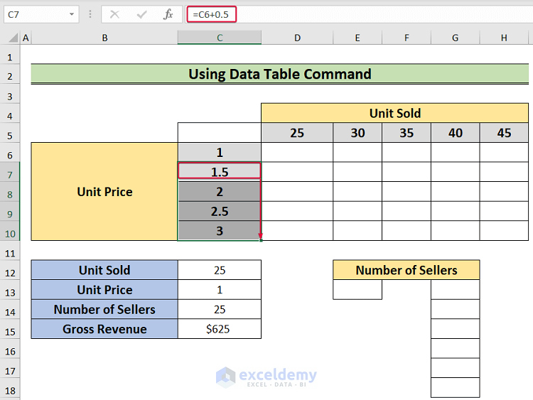
• Enter the following formula in C7.

• Press Enter.

• Drag down the Fill Handle to see the result in the rest of the cells.

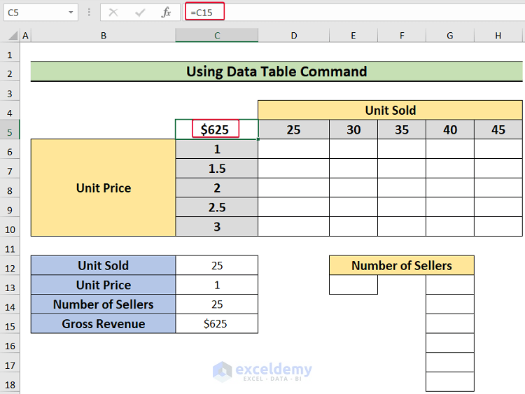
• Choose C5 cell and enter:

• Press Enter.

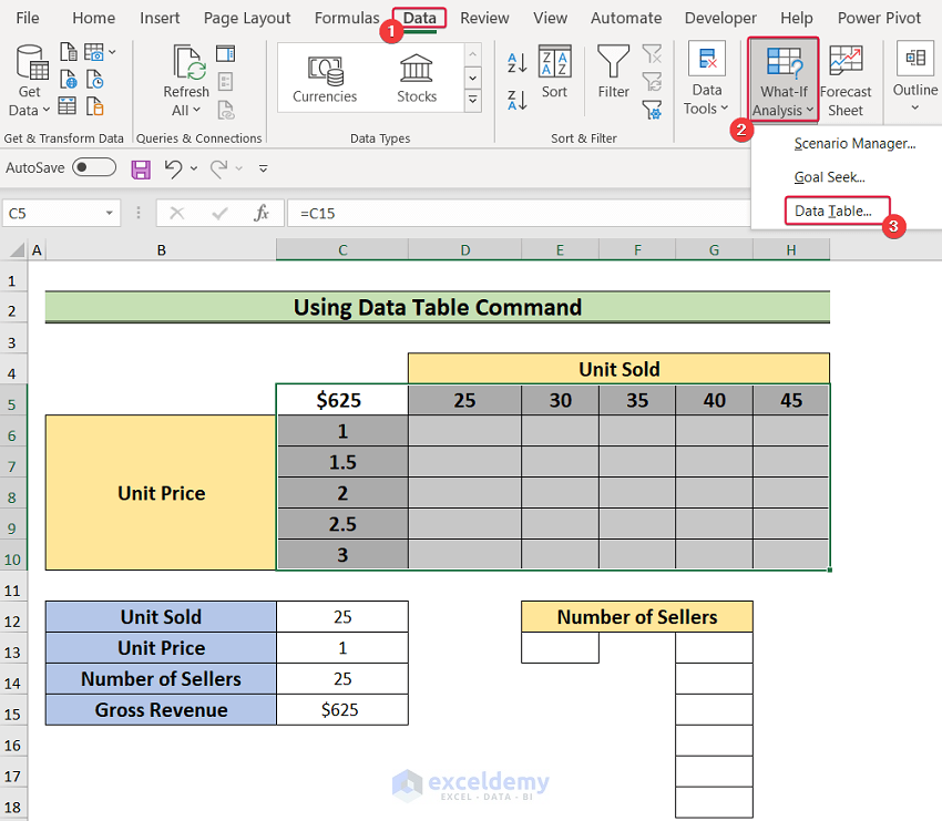
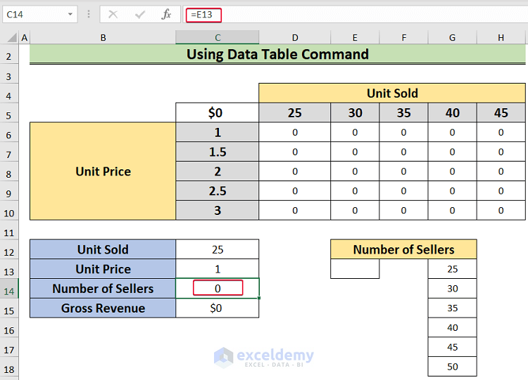
• Select C5:H10.
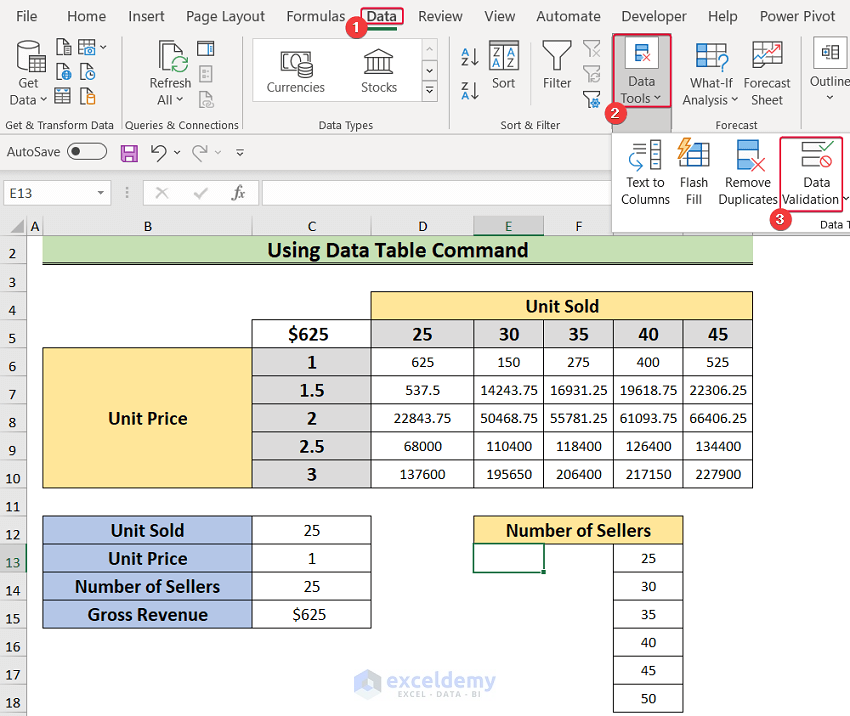
• Go to the Data tab.
• Select Data Table in What-If Analysis.

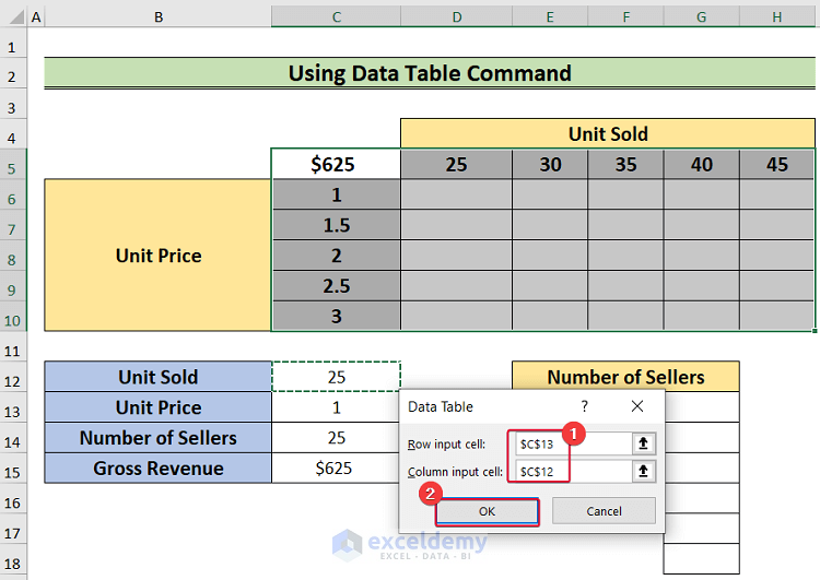
• Select C13 as Row input cell and C12 as Column input cell.
• Click OK.

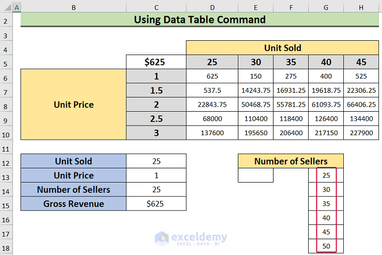
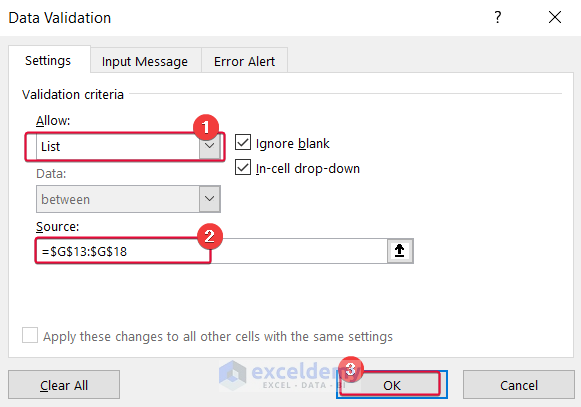
• Enter the list with the number of sellers in G13:G18.

• Select E13 and go to the Data tab.
• In Data Tools, select Data Validation.

• Select List in Allow.
• Select G13:G18 as Source.
• Click OK.

• Select C14 and enter:

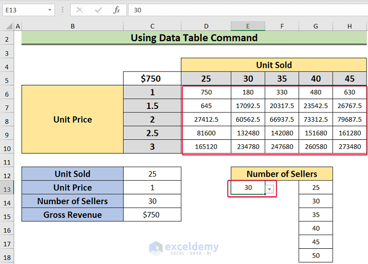
• Press Enter.

The value of E13 in the drop-down list changes and the values within the data table will also change.

Download Practice Workbook

Download the practice workbook here.

Related Articles

• How to Create One Variable Data Table Using What-If Analysis
• How to Create a 4-Variable Data Table in Excel

<< Go Back to Data Table in Excel | What-If Analysis in Excel | Learn Excel