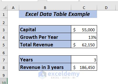
Example of Excel Data Table (6 Criteria)

We’re going to use the sample information, containing the values for Capital, Growth Per Year, Total Revenue, Years, and Revenue in Years.

Types of an Excel Data Table

Type 1 – One-Variable Data Table

One variable data table allows testing a series of values for a single input cell; it can be either the Row input cell or Column input cell and shows how those values change the result of a related formula.

It is best suited when you want to see how the eventual result changes when you change the input variables.

Type 2 – Two-Variable Data Table

A two-variable data table allows testing a series of values for a double input cell; You can use both the Row input cell and Column input cell and shows how changing two input values of the same formula changes the output

It is best suited when you want to see how the eventual result changes when you change two input variables.

Examples of Excel Data Tables

Example 1 – One Variable Data Table for Generating Total Revenue

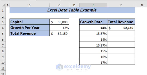
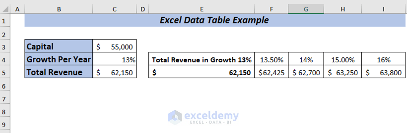
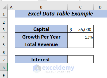
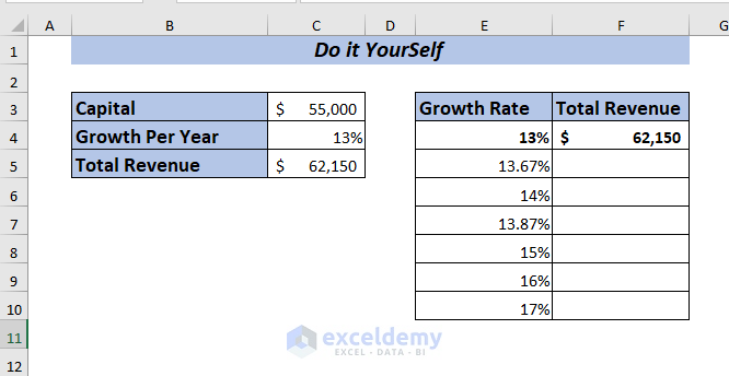
We want to observe the total revenue changes if we use different growth percentages. We have the information of Capital and Growth Per Year of the company. We want to know how the Total Revenue will change for the given percentages.

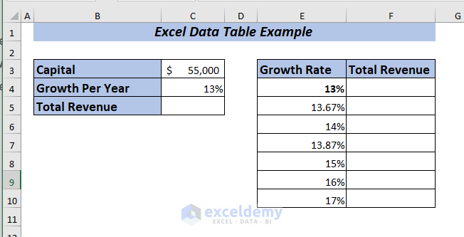
By using the value of Capital and Growth Per Year, we’ll determine the Total Revenue.

In cell C5, use the following formula.

=C3+C3*C4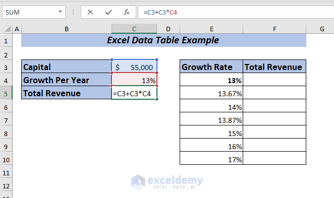

We multiplied the Capital with the Growth Per Year and then added the result with the Capital to get the Total Revenue.

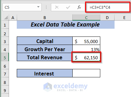
Press Enter, and you will get the Total Revenue for the year with 13% growth.

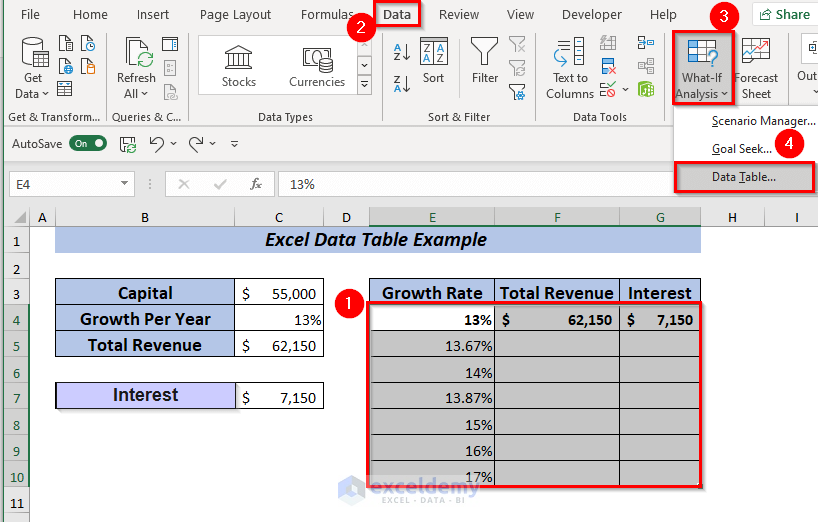
We want to perform a What-If-Analysis to see how the Total Revenue will change if we use the Growth Per Year ranging from 13% to 17% depending on the Capital amount of the company.

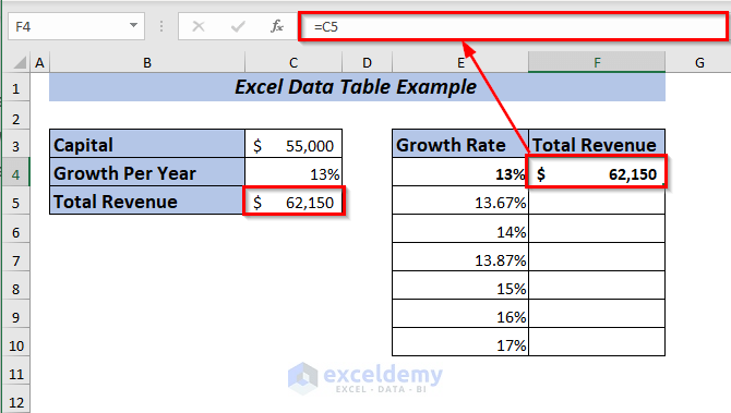
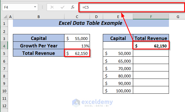
To apply one variable data table, place the formula of Total Revenue in cell F4.

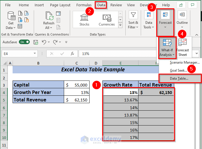
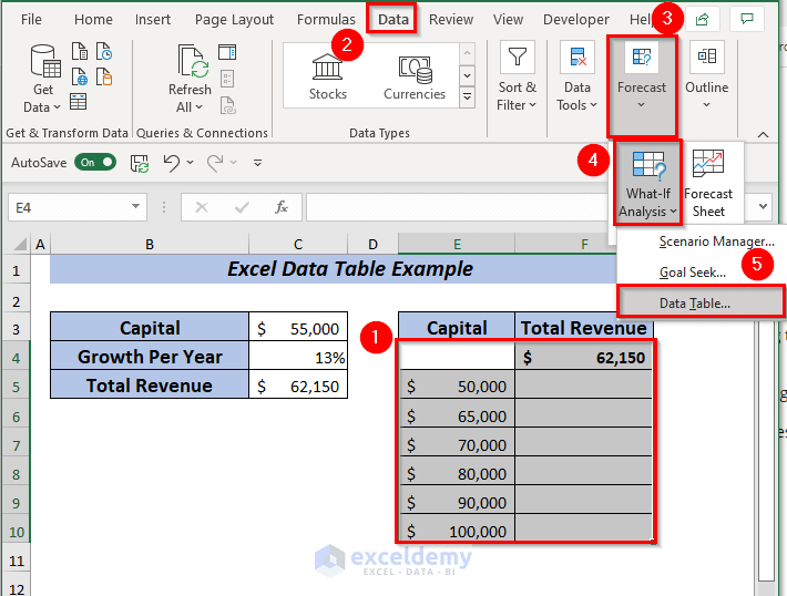
Select the range E4:F10 to apply the data table.
Open the Data tab and select Forecast.
Go to What-If-Analysis and select Data Table.

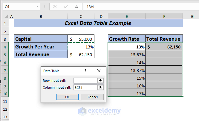
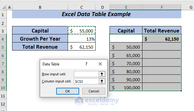
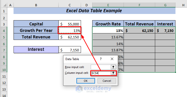
A dialog box will pop up.

Select any input cell. We want to see the changes in the column depending on growth per year. We selected C4 in the Column input cell box.
Click OK.

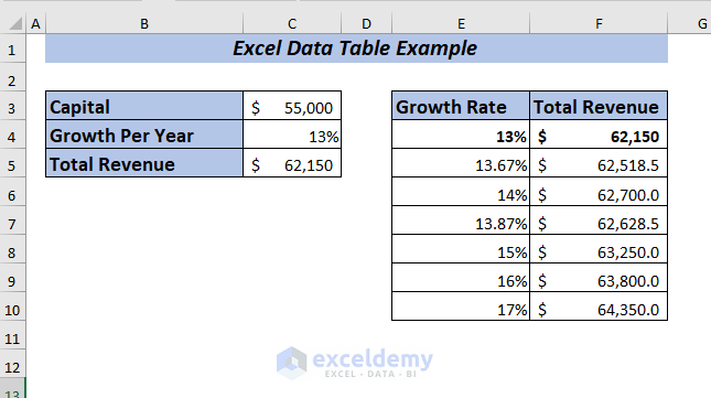
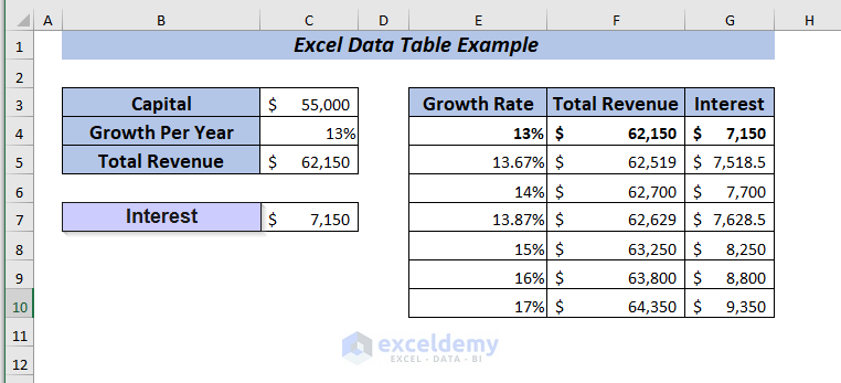
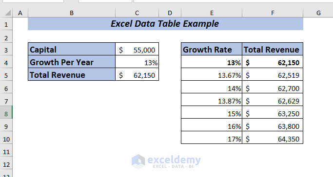
Result

You will get the Total Revenue for all the selected percentages.

Example 2 – One Variable Data Table for Observing Revenue Change

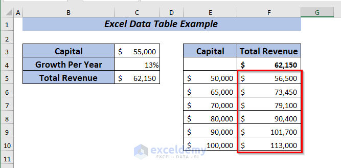
We will show you how the Total Revenue will change for Capital ranging from 50,000 to 100,000 while keeping the Growth Per Year at 13%.

To apply one variable data table, place the formula of Total Revenue in cell F4.

Insert the formula in cell F4.

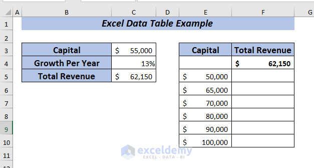
Select range E4:F10 to apply the data table.
Open the Data tab and go to Forecast.
Go to What-If-Analysis and select Data Table.

A dialog box will pop up.
Select any input cell. We want to see the changes in the column depending on the capital. We selected C3 in the Column input cell and clicked OK.

Result

You will get the Total Revenue for all the selected capitals at a glance.

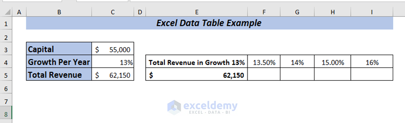
Example 3 – Row-Oriented Data Table

Place the formula in cell E5.
Put the values in a row while keeping one empty row below.

Select range E4:I5 to apply the data table.
Open the Data tab and go to Forecast.
Go to What-If-Analysis and select Data Table.

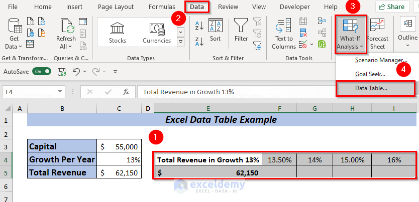
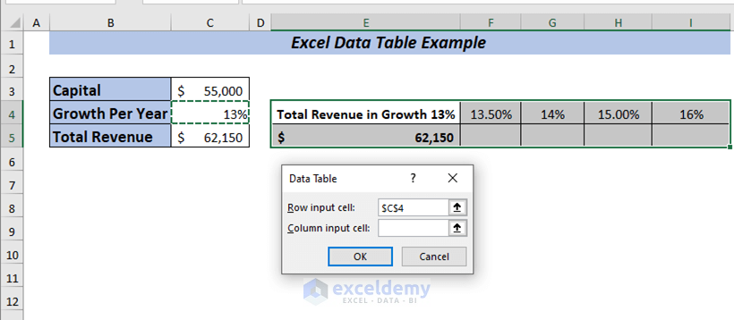
A dialog box will pop up.

Select any input cell. We want to see the changes in a row depending on percentages of growth per year. We selected C4 in the Row input cell and clicked OK.

Result

You will get the Total Revenue for all the selected percentages.

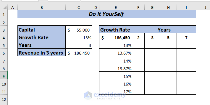
Example 4 – Two-Variable Data Table

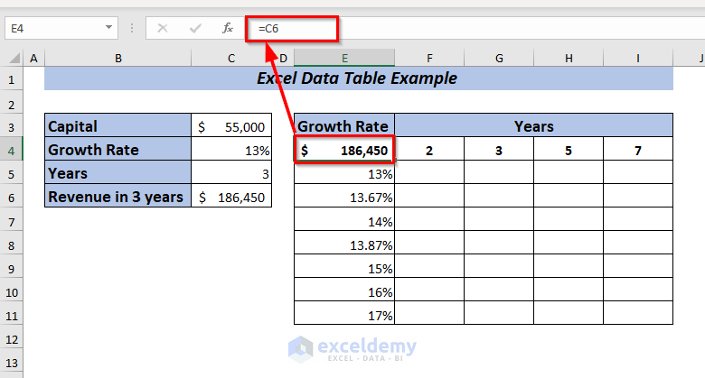
We’ve modified the dataset a bit, given below.

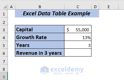
To calculate Revenue in 3 years:

In cell C5, use the following formula.

=(C3+C3*C4)*C5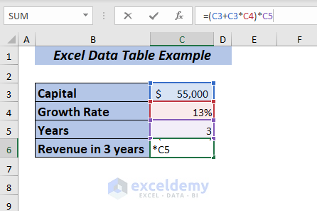

We have multiplied the Capital with the Growth Per Year and added the result with the Capital, then multiplied it by Years to get the Revenue in 3 years.

Press Enter, and you will get the Revenue in 3 years with 13% growth.

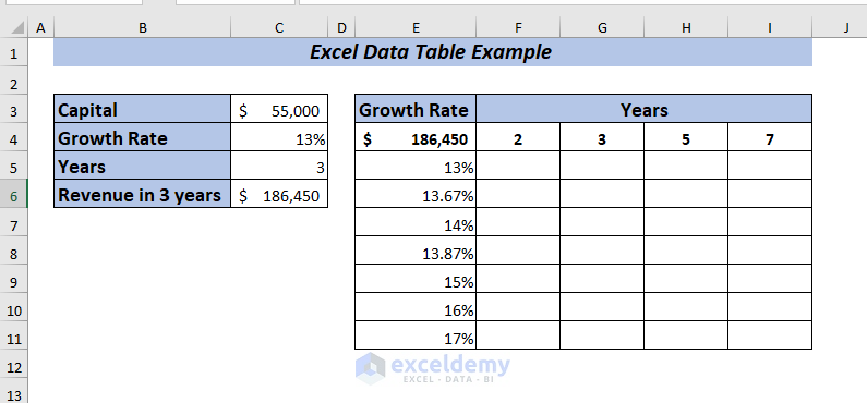
We want to perform a What-If-Analysis to see how the Revenue will change in different Years with Growth Per Year ranging from 13% to 17% depending on the Capital amount of the company.

To apply a two-variable data table, place the Total Revenue in cell E4.

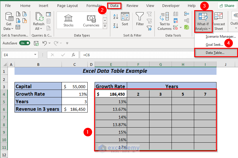
Select range E4:I11 to apply the data table.
Open the Data tab and go to Forecast.
Go to What-If-Analysis and select Data Table.

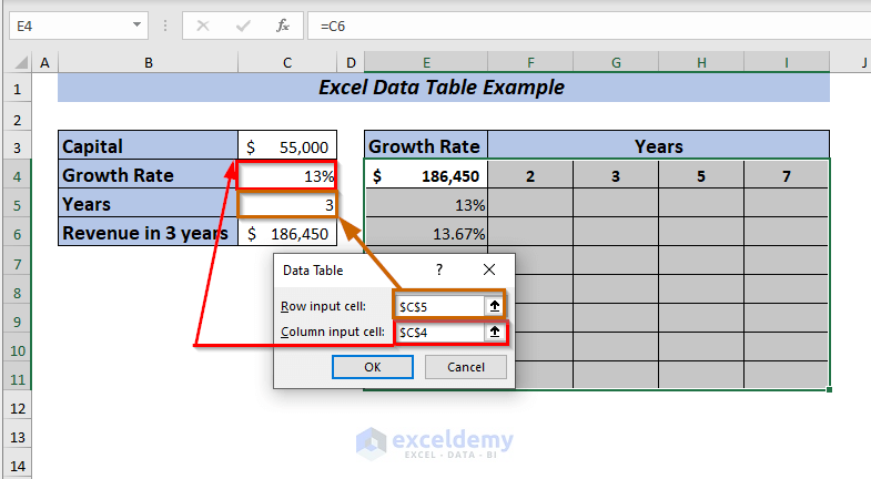
A dialog box will pop up.

Select C5 in the Row input cell because we kept the years in the row range F4:H4.
Select C4 in the Column input cell, as we kept the Growth Rate in a column range of E5:E11.
Click OK.

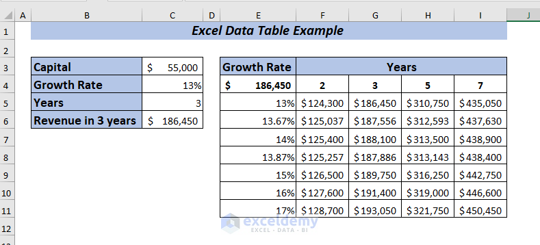
Result

You will get the Revenue for all the selected percentages and years.

Example 5 – Compare Multiple Results Using a Data Table

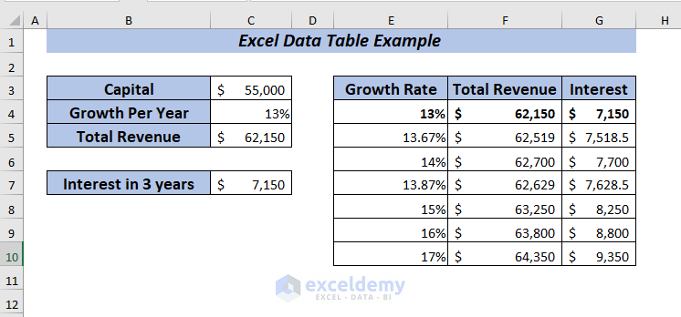
Here’s a comparison between Revenue and Interest using Data Table. We’re going to use the information given in the dataset below.

In cell C5, use the following formula for Total Revenue:

=C3+C3*C4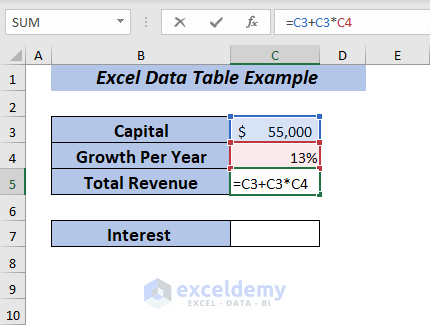

We multiplied the Capital with the Growth Per Year and then added the result with the Capital to get the Total Revenue.

Press Enter, and you will get the Total Revenue for the year with 13% growth.

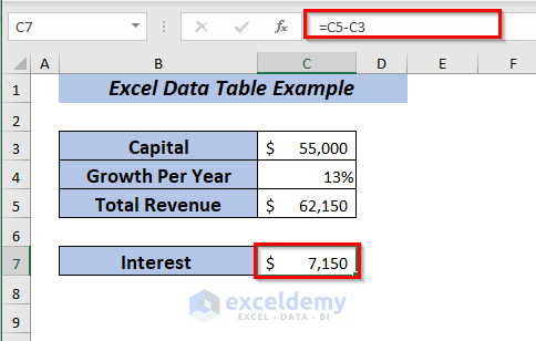
In cell C5, use the following formula for the Interest.

=C5-C3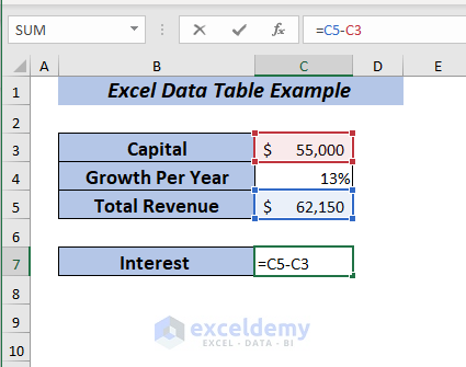

We subtracted the Capital from the Total Revenue to get the Interest.

Press Enter.

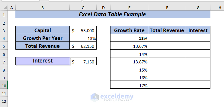
We will compare the Total Revenue and Interest using the data table.
Change the Growth Per Year ranging from 13% to 17% while the Capital amount is $55,000.

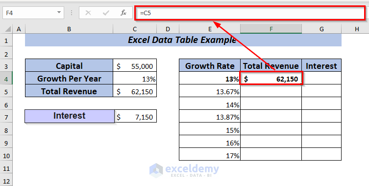
Place the formula for Total Revenue in cell F4.

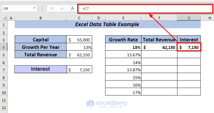
Place the formula for Interest in cell G4.

Select the range E4:G10 to apply the data table.
Open the Data tab and go to Forecast.
Go to What-If-Analysis and select Data Table.

A dialog box will pop up.
Select the input cell. We want to see the changes in the column depending on growth per year. We selected C4 in the Column input cell and pressed OK.

Result

You will get the Total Revenue and Interest for all the selected percentages.

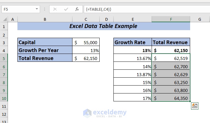
Example 6 – Example of Data Table Modifications

Case 6.1 – Edit the Data Table

We’ve taken a dataset where the data table is already applied to show you an example of editing an Excel data table.

Select the data table range from where you want to replace or edit data. We selected the range F4:F10.

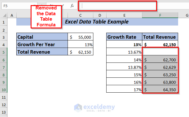
Remove the data table formula from any cell.

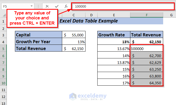
Insert the value of your choice and press Ctrl + Enter.

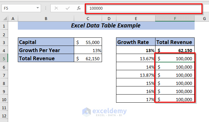
Result

The inserted same value will be in all the selected cells.

Case 6.2 – Delete the Data Table

We’re going to use the dataset given below.

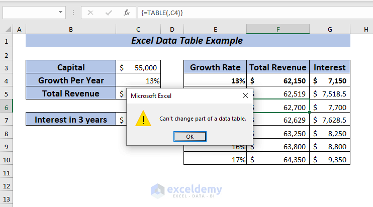
If you try to delete any cell from the data table then it will show you a warning message which is Can’t change part of a data table.

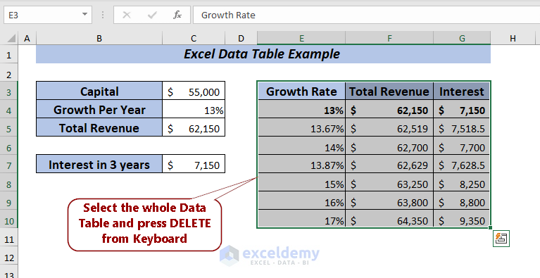
Select the entire range of the data table. We selected the cell range E3:G10.
Press Delete from the keyboard.

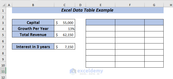
The entire data is deleted.

You also can use the Context Menu to delete the data table.

Select the entire range of the data table. We selected the cell range E3:G10.

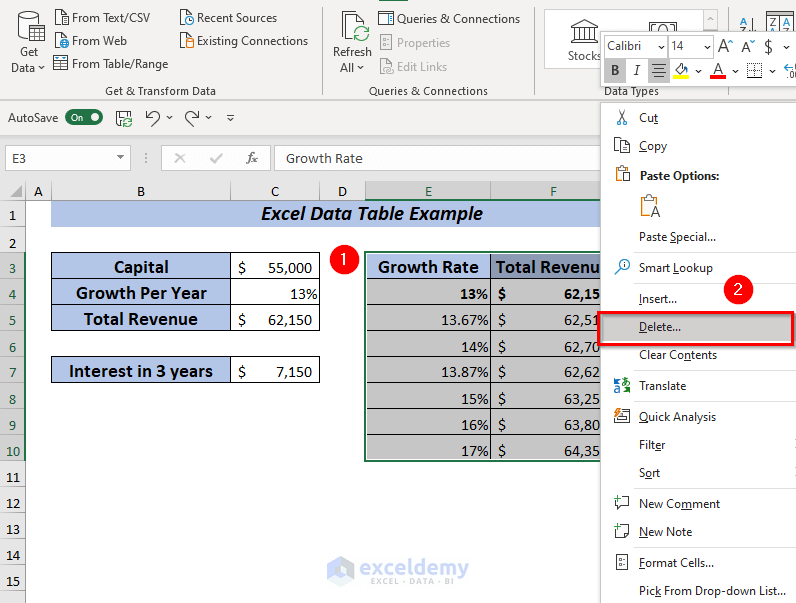
Right-click on the selection and pick Delete.
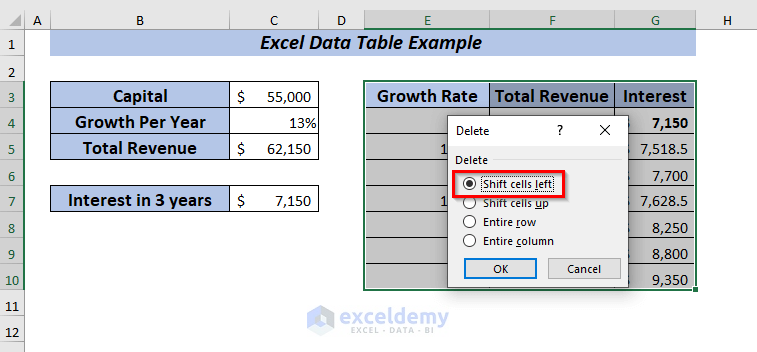
A dialog box will appear. Select any Delete option of your choice and click OK.

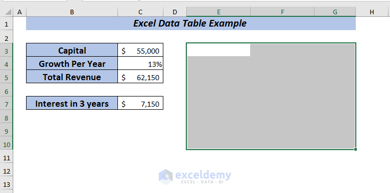
The data table is deleted.

Things To Remember

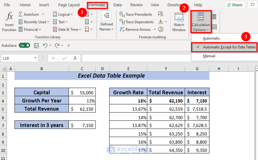
In your data table if you have multiple variable values and formulas that may slow down your Excel, then you can disable automatic recalculations in that and all other data tables which will speed up recalculations of the entire workbook.

Open Formulas tab >> From Calculation Options >> Select Automatic Except Data Tables.