Data tables are important parts of the Excel What-If Analysis feature to perform the sensitivity analysis of a business model. It is one of the most underutilized features in Excel. Are you having trouble creating a data table in Excel? In this article, I am going to explain how to create one variable data table using What-If Analysis. Let’s get started!
What Is a Data Table in Excel?
We can think of a data table as a dynamic range of cells that summarizes formula cells for varying input cells. Creating a data table is easy. Data tables have some limitations. In particular, a data table can deal with only one or two input cells at a time. We shall make clear the limitations of data tables in this article. You may be confused about a data table with a standard table. We can create a standard table by choosing this command: Insert >> Tables >> Table. These two tables are completely different. There is no relationship between these two tables.
In a one-variable data table, we use a single cell as the input in the data table. The values of the input may change and for different values of the input, the data table will display different results. We have to create a layout by ourselves, manually. Excel does not provide anything that will create the layout automatically. After that, we will apply the What If Analysis feature and specify a worksheet cell that contains the input value to complete our data table.
Step 1: Create a Layout of One Variable Data Table in Excel
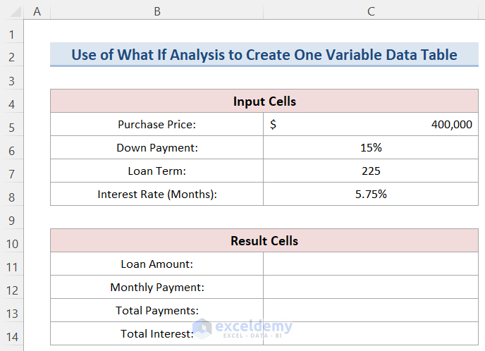
In this example, we have used the mortgage loan worksheet that we have used in the What-If Analysis Example article. The goal of this article is to create a data table. So that it will display the values of the four formula cells (loan amount, monthly payment, total payments, and total interest) for different interest rates ranging from 6.5% to 8.5%, in 0.25% increments. In order to do so, follow the steps below.
- First, we need to calculate the Result Cells by using simple Excel arithmetic formulas and functions. But these formulas are not part of our one variable data table.
- To calculate the result cells, select cell C11 and type the following formula.
=C5*(1-C6)- Then, press Enter and it will calculate the Loan Amount.

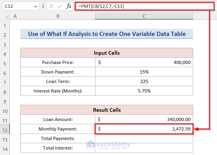
- After that, select cell C12 and type the following formula.
=PMT(C8/12,C7,-C11)- Now, press Enter and it will calculate the Monthly Payment.
- Select cell C13 and type the following formula.
=C12*C7- Next, press Enter and it will calculate the Total Payments.

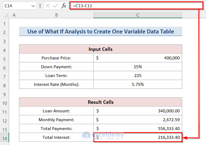
- Moreover, select cell C14 and type the following formula.
=C13-C11- Hence, press Enter and it will calculate the Total Interest.
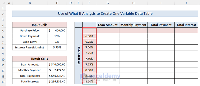
- Next, we need to create a layout like the following image where the values of the single input cell will be the interest rate in cells (F6:F14). Cell F5 will be empty, (G5:J5) cells will be the reference cells, and (G6:J14) cells will be used for the results of the one variable data table given by Excel.
- Now, type the interest rates starting from 50% in increments of .25% in the cells (F6:F14).
- To reference values in cells (G5:J5), select cell G5 and type the following formula.
=C11- Now, press Enter.

- After that, select cell H5 and type the following formula.
=C12- Next, press Enter.
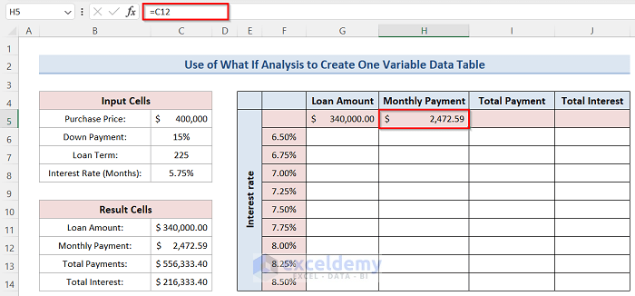
- Furthermore, select cell I5 and type the following formula.
=C13- Then, press Enter.

- Lastly, select cell J5 and type the following formula.
=C14- Then, press Enter.

- Finally, our layout is ready to create the one variable data table using the What If Analysis.

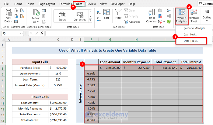
Step 2: Applying What If Analysis to One Variable Data Table
Our next task is to apply the What If Analysis feature to our layout.
- Firstly, select range F5:J14 >> Go to the Data tab >> Select the What If Analysis feature >> Choose Data Table from the options.
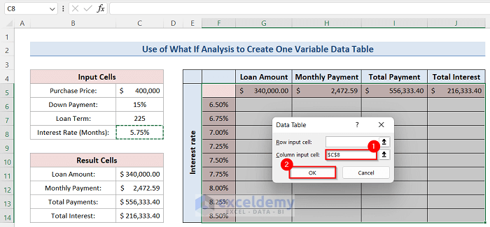
Step 3: Specifying Input Values for What If Analysis
Our final task is to specify the worksheet cell that contains the input value.
- After selecting the Data Table from the options, a Data Table dialog box will open.
- Select cell $C$8 in the Column input cell and click OK like the below one. The Row input cell will be blank.
Finally, we will see an output like the following figure where Excel will give the one variable data table for our example.

If you validate the contents of the cells of the data table, you’ll find that the data is generated with a multi-cell array formula: {=TABLE(,C8)}.

Things to Remember
- You can create a one-variable table vertically (what we’ve done in this example) or horizontally. After placing the values of the input cell in a row, we have to enter the input cell reference in the Row Input Cell field of the Data Table dialog box.
- Creating the layout manually is the most important part of one variable data table. If you make a mistake in this step, you will find errors in your result.
Download Practice Workbook
You can download the Excel workbook from here.
Conclusion
Hence, follow the above-described steps. Thus, you can easily learn how to create one variable data table using What If Analysis. Hope this will be helpful. Follow our website for more articles like this. Don’t forget to drop your comments, suggestions, or queries in the comment section below.
Related Articles
- How to Create a Two-Variable Data Table in Excel
- How to Create Data Table with 3 Variables
- How to Create a 4-Variable Data Table in Excel
<< Go Back to Data Table in Excel | What-If Analysis in Excel | Learn Excel
Get FREE Advanced Excel Exercises with Solutions!
