How to Timesheet Formula in Excel: 5 Methods

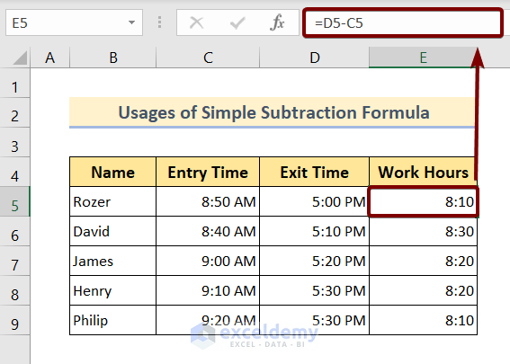
Method 1 – Excel Timesheet Formula: Using Simple Subtraction

Apply the simple arithmetic subtraction formula within this Excel timesheet. To do that, follow the steps below:

❶ First of all type of formula is below within cell E5.

❷ Press the ENTER button to execute the subtraction formula.

❸ Drag the Fill Handle icon to the end of the Work Hours column.

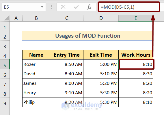
Method 2 – Excel Timesheet Formula: Using MOD Function

Instead of using the simple arithmetic subtraction formula, we can use the MOD function. Use the subtraction formula inside the MOD function within its argument list.

The MOD function has two arguments in total. Insert the subtraction formula in place of the first argument, and the second argument requires a divider value. Which will be 1 for this instance.

Now follow the steps below to learn the procedure:

❶ Select cell E5 to insert the formula below:

❷ Press the ENTER button.

❸ Drag the Fill Handle icon to the end of the Work Hours column.

That’s all.

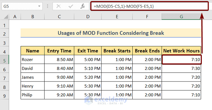
Method 3 – Excel Timesheet Formula: Using MOD Function Considering Break

To calculate the Net Work Hours, we must subtract the break period from the total office time period. So, we will use two MOD functions in total.

The first MOD function will return the total office work period, whereas the second MOD function will return the total break period. By subtracting these two results, we can easily get the Net Work Hours by each of the employees.

❶ Type the timesheet formula below within cell G5.

❷ Press the ENTER button.

❸ Daw the Fill Handle icon to the end of the Net Work Hours column.

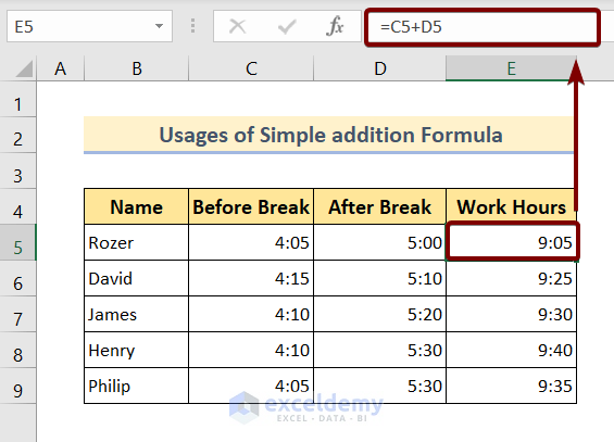
Method 4 – Excel Timesheet Formula: Using Simple Addition Formula

We divided the work hour count into two categories. Those are the total work hours before the break and, again, the total work hours after the break.

Now we can calculate the total work hours simply by adding work hours before the break to those after the break.

❶ Type the formula below within cell E5.

❷ Press the ENTER button.

❸ Pull the Fill Handle icon to the bottom of the Work Hours column.

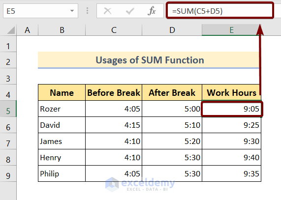
Method 5 – Excel Timesheet Formula: Using SUM Function

When there is only a little cell reference to add, we can use either the simple addition formula or the formula with the SUM function.

But when you have to sum up a large number of cell references, then there’s no alternative to using the SUM function.

❶ Select cell E5 and type the formula below:

❷ Press ENTER.

❸ Draw the Fill Handle icon at the end of the Work Hours column.

Things to Remember

As you work with the timesheet, always set the cell format to Time.

Download the Practice Workbook

You can download the Excel file from the link below and practice along with it.

Aging Formula in Excel: Knowledge Hub

<< Go Back to Formula List | Learn Excel